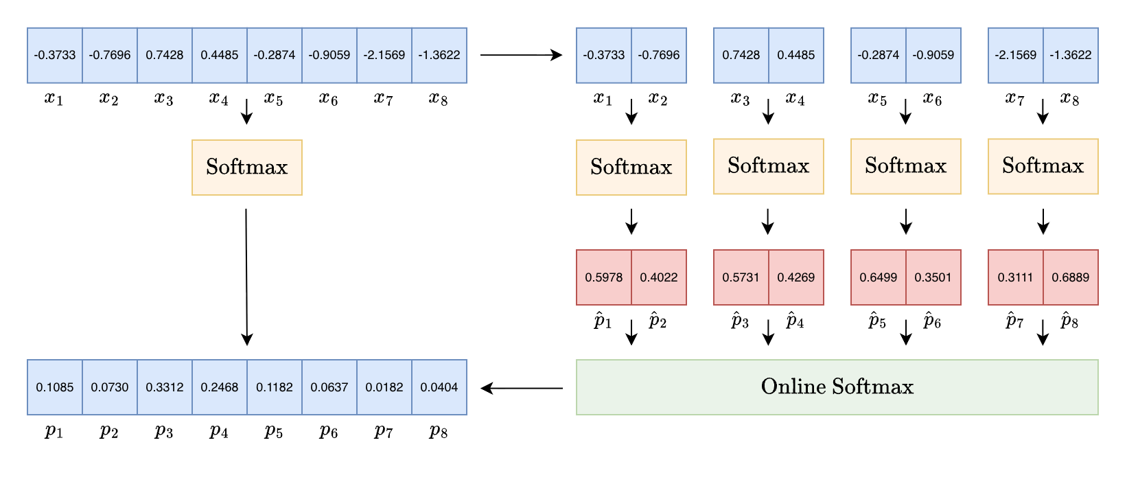
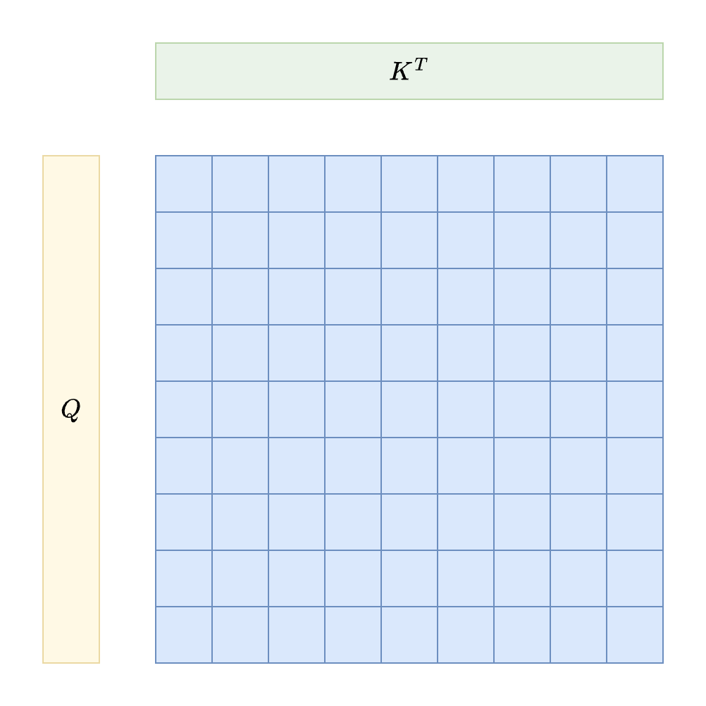
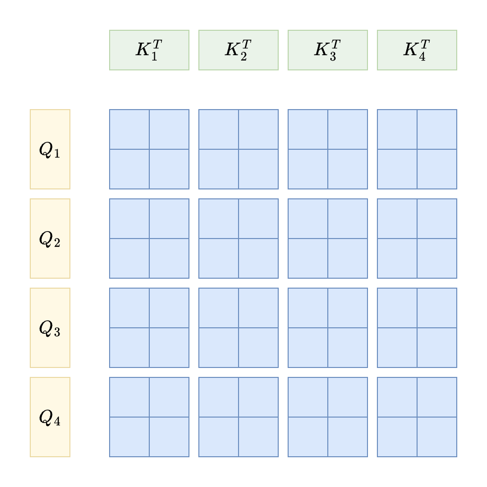
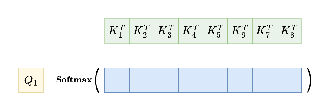
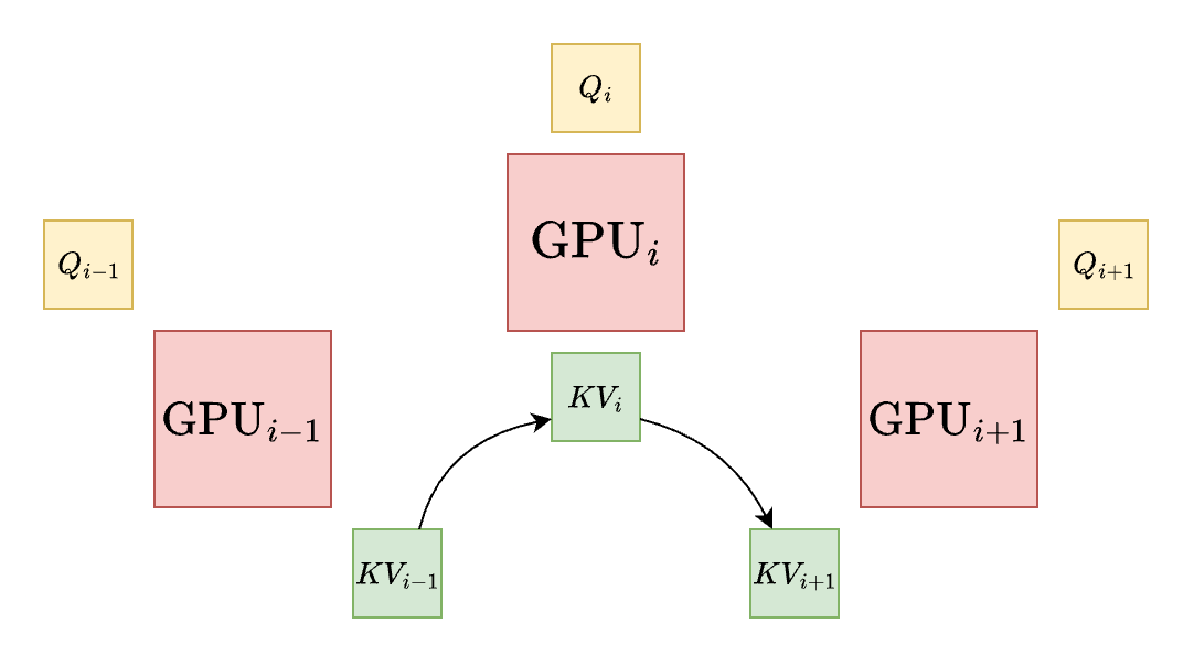
<?xml version="1.0" encoding="utf-8"?><feed xmlns="http://www.w3.org/2005/Atom" xml:lang="en"><generator uri="https://jekyllrb.com/" version="4.4.1">Jekyll</generator><link href="https://umutkavakli.github.io/feed.xml" rel="self" type="application/atom+xml"/><link href="https://umutkavakli.github.io/" rel="alternate" type="text/html" hreflang="en"/><updated>2026-09-14T00:29:28+00:00</updated><id>https://umutkavakli.github.io/feed.xml</id><title type="html">blank</title><subtitle>A simple, whitespace theme for academics. Based on [*folio](https://github.com/bogoli/-folio) design. </subtitle><entry><title type="html">Online Softmax in Attention Mechanism</title><link href="https://umutkavakli.github.io/blog/2026/online-softmax/" rel="alternate" type="text/html" title="Online Softmax in Attention Mechanism"/><published>2026-01-10T14:49:00+00:00</published><updated>2026-01-10T14:49:00+00:00</updated><id>https://umutkavakli.github.io/blog/2026/online-softmax</id><content type="html" xml:base="https://umutkavakli.github.io/blog/2026/online-softmax/"><![CDATA[<p>As sequences get longer in Transformer models, the standard approach to processing data becomes incredibly expensive and often exceeds GPU memory limits. Instead of processing the entire sequence as a single large block, we can split it into smaller chunks and merge them incrementally. This method ensures that sequence generation remains efficient and produces exact results while keeping memory usage under control.</p> <d-figure> <img src="/assets/img/posts/2026-01-10-online-softmax/onlinesoftmax.png" style="width: 100%; display: block; margin: auto;"/> </d-figure> <p>The <a href="https://en.wikipedia.org/wiki/Softmax_function">softmax</a> function is an crucial part of modern deep learning. It is especially important for the attention mechanism used in Transformer models. In self-attention, softmax converts raw similarity scores into a probability distribution. This distribution tells the model how much focus to put on each token in a sequence. We usually define scaled dot product attention like this:</p> \[\text{Attention(Q, K, V)} = \text{softmax}\left(\frac{QK^T}{\sqrt{d_k}} \right) V\] <p>When we calculate the dot product of queries and keys, we get an $N \times N$ a sequence of length $N$. This creates a major problem because the time and memory needed grow at a quadratic rate $O(N^2)$:</p> <d-figure> <img src="/assets/img/posts/2026-01-10-online-softmax/attention.png" style="width: 75%; display: block; margin: auto;"/> </d-figure> <p>For very long sequences, a single GPU cannot store the entire attention matrix. The Ring Attention paper <d-cite key="liu2023ring"></d-cite> highlights just how extreme this memory demand can be:</p> <blockquote> <p>To put the memory demand in perspective, even when dealing with a batch size of 1, processing 100 million tokens requires over <strong>1000 GB</strong> of memory for a modest model with a hidden size of 1024.</p> </blockquote> <p>To solve this, we can split the attention matrix into smaller blocks and run calculations on those blocks individually <d-cite key="dao2022flashattention,liu2023blockwise"></d-cite>:</p> <d-figure> <img src="/assets/img/posts/2026-01-10-online-softmax/attention2.png" style="width: 75%; display: block; margin: auto;"/> </d-figure> <p>Processing in blocks is a great idea, but the standard softmax function makes it difficult because it needs the sum of every element in the sequence to calculate the denominator.</p> <h2 id="naive-softmax">Naive Softmax</h2> <p>The standard softmax formula is defined as:</p> \[\text{Softmax}(x_i) = \frac{\exp(x_i)}{\sum_{j=1}^{N} \exp(x_j)}\] <p>We can write a simple version of this in PyTorch:</p> <div class="language-python highlighter-rouge"><div class="highlight"><pre class="highlight"><code><span class="kn">import</span> <span class="n">torch</span>

<span class="k">def</span> <span class="nf">naive_softmax</span><span class="p">(</span><span class="n">x</span><span class="p">:</span> <span class="n">torch</span><span class="p">.</span><span class="n">Tensor</span><span class="p">)</span> <span class="o">-&gt;</span> <span class="n">torch</span><span class="p">.</span><span class="n">Tensor</span><span class="p">:</span>
    <span class="k">return</span> <span class="n">x</span><span class="p">.</span><span class="nf">exp</span><span class="p">()</span> <span class="o">/</span> <span class="n">x</span><span class="p">.</span><span class="nf">exp</span><span class="p">().</span><span class="nf">sum</span><span class="p">()</span>
</code></pre></div></div> <p>If we compare this naive function to the official PyTorch version, the results look identical for small numbers:</p> <div class="language-python highlighter-rouge"><div class="highlight"><pre class="highlight"><code><span class="n">x</span>         <span class="o">=</span> <span class="n">torch</span><span class="p">.</span><span class="nf">randn</span><span class="p">(</span><span class="mi">8</span><span class="p">)</span>
<span class="n">reference</span> <span class="o">=</span> <span class="n">torch</span><span class="p">.</span><span class="nf">softmax</span><span class="p">(</span><span class="n">x</span><span class="p">,</span> <span class="n">dim</span><span class="o">=-</span><span class="mi">1</span><span class="p">)</span>
<span class="n">naive</span>     <span class="o">=</span> <span class="nf">naive_softmax</span><span class="p">(</span><span class="n">x</span><span class="p">)</span>

<span class="nf">print</span><span class="p">(</span><span class="sa">f</span><span class="sh">"</span><span class="s">Torch: </span><span class="si">{</span><span class="n">reference</span><span class="si">}</span><span class="sh">"</span><span class="p">)</span>
<span class="nf">print</span><span class="p">(</span><span class="sa">f</span><span class="sh">"</span><span class="s">Naive: </span><span class="si">{</span><span class="n">naive</span><span class="si">}</span><span class="sh">"</span><span class="p">)</span>
<span class="nf">print</span><span class="p">(</span><span class="sa">f</span><span class="sh">"</span><span class="s">allclose: </span><span class="si">{</span><span class="n">torch</span><span class="p">.</span><span class="nf">allclose</span><span class="p">(</span><span class="n">reference</span><span class="p">,</span> <span class="n">naive</span><span class="p">)</span><span class="si">}</span><span class="sh">"</span><span class="p">)</span>
</code></pre></div></div> <div class="language-python highlighter-rouge"><div class="highlight"><pre class="highlight"><code><span class="c1"># Output
</span><span class="n">Torch</span><span class="p">:</span> <span class="nf">tensor</span><span class="p">([</span><span class="mf">0.1085</span><span class="p">,</span> <span class="mf">0.0730</span><span class="p">,</span> <span class="mf">0.3312</span><span class="p">,</span> <span class="mf">0.2468</span><span class="p">,</span> <span class="mf">0.1182</span><span class="p">,</span> <span class="mf">0.0637</span><span class="p">,</span> <span class="mf">0.0182</span><span class="p">,</span> <span class="mf">0.0404</span><span class="p">])</span>
<span class="n">Naive</span><span class="p">:</span> <span class="nf">tensor</span><span class="p">([</span><span class="mf">0.1085</span><span class="p">,</span> <span class="mf">0.0730</span><span class="p">,</span> <span class="mf">0.3312</span><span class="p">,</span> <span class="mf">0.2468</span><span class="p">,</span> <span class="mf">0.1182</span><span class="p">,</span> <span class="mf">0.0637</span><span class="p">,</span> <span class="mf">0.0182</span><span class="p">,</span> <span class="mf">0.0404</span><span class="p">])</span>
<span class="n">allclose</span><span class="p">:</span> <span class="bp">True</span>
</code></pre></div></div> <p>However, this naive version is <strong>not stable</strong>. When the input values are large, the exponential function grows too fast and causes a numerical overflow. This results in “nan” errors in naive softmax:</p> <div class="language-python highlighter-rouge"><div class="highlight"><pre class="highlight"><code><span class="nf">naive_softmax</span><span class="p">(</span><span class="n">x</span> <span class="o">*</span> <span class="mi">1000</span><span class="p">)</span>
</code></pre></div></div> <div class="language-python highlighter-rouge"><div class="highlight"><pre class="highlight"><code><span class="c1"># Output
</span><span class="nf">tensor</span><span class="p">([</span><span class="mf">0.</span><span class="p">,</span> <span class="mf">0.</span><span class="p">,</span> <span class="n">nan</span><span class="p">,</span> <span class="n">nan</span><span class="p">,</span> <span class="mf">0.</span><span class="p">,</span> <span class="mf">0.</span><span class="p">,</span> <span class="mf">0.</span><span class="p">,</span> <span class="mf">0.</span><span class="p">])</span>
</code></pre></div></div> <h2 id="safe-softmax">Safe Softmax</h2> <p>Softmax has the <strong>shift invariance</strong> property. This means that if we add or subtract the same constant from every input, the output stays the same. We can use this to keep our numbers small and manageable. By subtracting the maximum value from the entire vector, we ensure that the largest exponent is exactly zero.</p> \[\begin{align*} \text{SafeSoftmax}(x_i) &amp;= \frac{\exp(x_i)}{\sum_{j=1}^{N} \exp(x_j)} \cdot \frac{\exp(- \max_{k=1}^{N} x_k)}{\exp(- \max_{k=1}^{N} x_k)} \\\\ &amp;= \frac{\exp(x_i - \max_{k=1}^{N} x_k)}{\sum_{j=1}^{N} \exp(x_j - \max_{k=1}^{N} x_k)} \end{align*}\] <p>By doing this, every exponent is less than or equal to zero, which completely prevents overflow. Here is how we implement it:</p> <div class="language-python highlighter-rouge"><div class="highlight"><pre class="highlight"><code><span class="k">def</span> <span class="nf">safe_softmax</span><span class="p">(</span><span class="n">x</span><span class="p">:</span> <span class="n">torch</span><span class="p">.</span><span class="n">Tensor</span><span class="p">)</span> <span class="o">-&gt;</span> <span class="n">torch</span><span class="p">.</span><span class="n">Tensor</span><span class="p">:</span>
    <span class="n">m</span> <span class="o">=</span> <span class="n">x</span><span class="p">.</span><span class="nf">max</span><span class="p">()</span>
    <span class="nf">return </span><span class="p">(</span><span class="n">x</span> <span class="o">-</span> <span class="n">m</span><span class="p">).</span><span class="nf">exp</span><span class="p">()</span> <span class="o">/</span> <span class="p">(</span><span class="n">x</span> <span class="o">-</span> <span class="n">m</span><span class="p">).</span><span class="nf">exp</span><span class="p">().</span><span class="nf">sum</span><span class="p">()</span>
</code></pre></div></div> <div class="language-python highlighter-rouge"><div class="highlight"><pre class="highlight"><code><span class="n">reference</span> <span class="o">=</span> <span class="n">torch</span><span class="p">.</span><span class="nf">softmax</span><span class="p">(</span><span class="n">x</span><span class="p">,</span> <span class="n">dim</span><span class="o">=-</span><span class="mi">1</span><span class="p">)</span>
<span class="n">safe</span>      <span class="o">=</span> <span class="nf">safe_softmax</span><span class="p">(</span><span class="n">x</span><span class="p">)</span>

<span class="nf">print</span><span class="p">(</span><span class="sa">f</span><span class="sh">"</span><span class="s">Torch: </span><span class="si">{</span><span class="n">reference</span><span class="si">}</span><span class="sh">"</span><span class="p">)</span>
<span class="nf">print</span><span class="p">(</span><span class="sa">f</span><span class="sh">"</span><span class="s">Safe: </span><span class="si">{</span><span class="n">safe</span><span class="si">}</span><span class="sh">"</span><span class="p">)</span>
<span class="nf">print</span><span class="p">(</span><span class="sa">f</span><span class="sh">"</span><span class="s">allclose: </span><span class="si">{</span><span class="n">torch</span><span class="p">.</span><span class="nf">allclose</span><span class="p">(</span><span class="n">reference</span><span class="p">,</span> <span class="n">safe</span><span class="p">)</span><span class="si">}</span><span class="sh">"</span><span class="p">)</span>
</code></pre></div></div> <div class="language-python highlighter-rouge"><div class="highlight"><pre class="highlight"><code><span class="c1"># Output
</span><span class="n">Torch</span><span class="p">:</span> <span class="nf">tensor</span><span class="p">([</span><span class="mf">0.1085</span><span class="p">,</span> <span class="mf">0.0730</span><span class="p">,</span> <span class="mf">0.3312</span><span class="p">,</span> <span class="mf">0.2468</span><span class="p">,</span> <span class="mf">0.1182</span><span class="p">,</span> <span class="mf">0.0637</span><span class="p">,</span> <span class="mf">0.0182</span><span class="p">,</span> <span class="mf">0.0404</span><span class="p">])</span>
<span class="n">Safe</span><span class="p">:</span> <span class="nf">tensor</span><span class="p">([</span><span class="mf">0.1085</span><span class="p">,</span> <span class="mf">0.0730</span><span class="p">,</span> <span class="mf">0.3312</span><span class="p">,</span> <span class="mf">0.2468</span><span class="p">,</span> <span class="mf">0.1182</span><span class="p">,</span> <span class="mf">0.0637</span><span class="p">,</span> <span class="mf">0.0182</span><span class="p">,</span> <span class="mf">0.0404</span><span class="p">])</span>
<span class="n">allclose</span><span class="p">:</span> <span class="bp">True</span>
</code></pre></div></div> <p>This version is also stable for large inputs:</p> <div class="language-python highlighter-rouge"><div class="highlight"><pre class="highlight"><code><span class="nf">safe_softmax</span><span class="p">(</span><span class="n">x</span> <span class="o">*</span> <span class="mi">1000</span><span class="p">)</span>
</code></pre></div></div> <div class="language-python highlighter-rouge"><div class="highlight"><pre class="highlight"><code><span class="c1"># Output
</span><span class="nf">tensor</span><span class="p">([</span><span class="mf">0.</span><span class="p">,</span> <span class="mf">0.</span><span class="p">,</span> <span class="mf">1.</span><span class="p">,</span> <span class="mf">0.</span><span class="p">,</span> <span class="mf">0.</span><span class="p">,</span> <span class="mf">0.</span><span class="p">,</span> <span class="mf">0.</span><span class="p">,</span> <span class="mf">0.</span><span class="p">])</span>
</code></pre></div></div> <h2 id="online-softmax">Online Softmax</h2> <p>In the attention mechanism, we apply softmax row by row. To calculate the denominator for a single query, we need to access every single key vector in that row. This global dependency is exactly what makes it hard to process the matrix in chunks:</p> <d-figure> <img src="/assets/img/posts/2026-01-10-online-softmax/attention3.png" style="width: 75%; display: block; margin: auto;"/> </d-figure> <p>Online softmax <d-cite key="milakov2018online"></d-cite> allows us to calculate the result step by step. If we track the local maximum $m$ and the local sum $d$ for each small block, we can update them as we move through the sequence. When we receive a new element $x_S$, we update our statistics like this:</p> \[\begin{align*} m_S &amp;\leftarrow \max(m_{S-1}, x_S) \\ d_S &amp;\leftarrow d_{S-1} \cdot\exp(m_{S-1} - m_S) + \exp(x_{S} - m_S) \end{align*}\] <details><summary>Click for the proof</summary> \[\begin{align*} m_S &amp;\leftarrow \max(m_{S-1}, x_S) \\ &amp;= \max(\max_{k=1}^{S-1} x_k, x_S) \\ &amp;= \max_{k=1}^{S} x_k \\\\ d_S &amp;\leftarrow d_{S-1} \cdot\exp(m_{S-1} - m_S) + \exp(x_{S} - m_S) \\ &amp;= \left(\sum_{j=1}^{S-1} \exp(x_j - {\color{red} \cancel{m_{S-1}}}) \right) \cdot \exp({\color{red} \cancel{m_{S-1}}} - m_S) + \exp(x_{S} - m_S) \\ &amp;= \left(\sum_{j=1}^{S-1} \exp(x_j - m_{S}) \right) + \exp(x_{S} - m_S) \\ &amp;= \sum_{j=1}^{S} \exp(x_j - m_{S}) \end{align*}\] </details> <p>This logic allows us to merge several local results into one global distribution. If we have $B$ blocks, each with its own max value $m_i$ and sum $d_i$, we can combine them by rescaling the local probabilities. This approach perfectly matches the standard softmax output:</p> \[\begin{align*} \text{OnlineSoftmax}(p_i, m_i, d_i) &amp;= \frac{p_i \cdot d_i \cdot \exp(m_i -\max_{k=1}^{B})}{\sum_{j=1}^B d_j \cdot \exp(m_j - \max_{k=1}^{B})} \\ \end{align*}\] <details><summary>Click for the proof</summary> \[\begin{align*} \text{OnlineSoftmax}(p_i, m_i, d_i) &amp;= \frac{p_i \cdot d_i \cdot \exp(m_i -\max_{k=1}^{B})}{\sum_{j=1}^B d_j \cdot \exp(m_j - \max_{k=1}^{B})} \\\\ &amp;= \frac{\frac{\exp(x_i - m_i)}{{\color{red} \cancel{d_i}}} \cdot {\color{red} \cancel{d_i}} \cdot \exp(m_i -\max_{k=1}^{B})}{\sum_{j=1}^B d_j \cdot \exp(m_j - \max_{k=1}^{B})} \\\\ &amp;= \frac{\exp(x_i - {\color{red} \cancel{m_i}}) \cdot \exp({\color{red} \cancel{m_i}} -\max_{k=1}^{B})}{\sum_{j=1}^B d_j \cdot \exp(m_j - \max_{k=1}^{B})} \\\\ &amp;= \frac{\exp(x_i -\max_{k=1}^{B})}{\sum_{j=1}^B d_j \cdot \exp(m_j - \max_{k=1}^{B})} \\\\ &amp;= \frac{\exp(x_i -\max_{k=1}^{B})}{\sum_{j=1}^B \left[\sum_{l=1}^{S_j} \exp(x_l - {\color{red} \cancel{m_i}}) \right] \cdot \exp({\color{red} \cancel{m_i}} - \max_{k=1}^{B})} \\\\ &amp;= \frac{\exp(x_i -\max_{k=1}^{B})}{\sum_{j=1}^N \exp(x_j - \max_{k=1}^{B})} \quad\quad\quad \left(N = \sum_{j=1}^{B} S_j \right) \\ \end{align*}\] </details> <p>We first need a modified version of safe softmax that returns the local maximum and the denominator sum:</p> <div class="language-python highlighter-rouge"><div class="highlight"><pre class="highlight"><code><span class="k">def</span> <span class="nf">safe_softmax2</span><span class="p">(</span><span class="n">x</span><span class="p">:</span> <span class="n">torch</span><span class="p">.</span><span class="n">Tensor</span><span class="p">)</span> <span class="o">-&gt;</span> <span class="n">torch</span><span class="p">.</span><span class="n">Tensor</span><span class="p">:</span>
    <span class="n">m</span> <span class="o">=</span> <span class="n">x</span><span class="p">.</span><span class="nf">max</span><span class="p">()</span>
    <span class="n">a</span> <span class="o">=</span> <span class="p">(</span><span class="n">x</span> <span class="o">-</span> <span class="n">m</span><span class="p">).</span><span class="nf">exp</span><span class="p">()</span> <span class="c1"># subtract maximum value
</span>    <span class="n">d</span> <span class="o">=</span> <span class="n">a</span><span class="p">.</span><span class="nf">sum</span><span class="p">()</span> <span class="c1"># normalization factor
</span>    <span class="k">return</span> <span class="n">a</span> <span class="o">/</span> <span class="n">d</span><span class="p">,</span> <span class="n">m</span><span class="p">,</span> <span class="n">d</span>
</code></pre></div></div> <p>Next, we create the online softmax function. It takes these local blocks and merges them by finding a global maximum and adjusting the sums accordingly:</p> <div class="language-python highlighter-rouge"><div class="highlight"><pre class="highlight"><code><span class="k">def</span> <span class="nf">online_softmax</span><span class="p">(</span>
    <span class="o">*</span><span class="n">blocks</span><span class="p">:</span> <span class="n">Tuple</span><span class="p">[</span><span class="n">torch</span><span class="p">.</span><span class="n">Tensor</span><span class="p">,</span> <span class="n">torch</span><span class="p">.</span><span class="n">Tensor</span><span class="p">,</span> <span class="n">torch</span><span class="p">.</span><span class="n">Tensor</span><span class="p">]</span>
<span class="p">)</span> <span class="o">-&gt;</span> <span class="n">torch</span><span class="p">.</span><span class="n">Tensor</span><span class="p">:</span>
    <span class="n">p_blocks</span><span class="p">,</span> <span class="n">m_blocks</span><span class="p">,</span> <span class="n">d_blocks</span> <span class="o">=</span> <span class="nf">zip</span><span class="p">(</span><span class="o">*</span><span class="n">blocks</span><span class="p">)</span>
    <span class="n">m_max</span> <span class="o">=</span> <span class="n">torch</span><span class="p">.</span><span class="nf">stack</span><span class="p">(</span><span class="n">m_blocks</span><span class="p">).</span><span class="nf">max</span><span class="p">()</span> <span class="c1"># get global maximum
</span>    <span class="n">d_total</span> <span class="o">=</span> <span class="nf">sum</span><span class="p">(</span> <span class="c1"># compute global normalizer
</span>        <span class="n">d</span> <span class="o">*</span> <span class="n">torch</span><span class="p">.</span><span class="nf">exp</span><span class="p">(</span><span class="n">m</span> <span class="o">-</span> <span class="n">m_max</span><span class="p">)</span>
        <span class="k">for</span> <span class="n">d</span><span class="p">,</span> <span class="n">m</span> <span class="ow">in</span> <span class="nf">zip</span><span class="p">(</span><span class="n">d_blocks</span><span class="p">,</span> <span class="n">m_blocks</span><span class="p">)</span>
    <span class="p">)</span>
    <span class="k">return</span> <span class="n">torch</span><span class="p">.</span><span class="nf">cat</span><span class="p">(</span>
        <span class="p">[</span>
            <span class="n">p</span> <span class="o">*</span> <span class="n">d</span> <span class="o">*</span> <span class="n">torch</span><span class="p">.</span><span class="nf">exp</span><span class="p">(</span><span class="n">m</span> <span class="o">-</span> <span class="n">m_max</span><span class="p">)</span> <span class="o">/</span> <span class="n">d_total</span>
            <span class="k">for</span> <span class="n">p</span><span class="p">,</span> <span class="n">m</span><span class="p">,</span> <span class="n">d</span> <span class="ow">in</span> <span class="nf">zip</span><span class="p">(</span><span class="n">p_blocks</span><span class="p">,</span> <span class="n">m_blocks</span><span class="p">,</span> <span class="n">d_blocks</span><span class="p">)</span>
        <span class="p">]</span>
    <span class="p">)</span>
</code></pre></div></div> <p>Finally, we can verify that splitting the input into four chunks and processing them with our online softmax function gives the correct result:</p> <div class="language-python highlighter-rouge"><div class="highlight"><pre class="highlight"><code><span class="n">blocks</span> <span class="o">=</span> <span class="p">[]</span>

<span class="k">for</span> <span class="n">chunk</span> <span class="ow">in</span> <span class="nf">list</span><span class="p">(</span><span class="n">x</span><span class="p">.</span><span class="nf">chunk</span><span class="p">(</span><span class="mi">4</span><span class="p">)):</span>
    <span class="n">blocks</span><span class="p">.</span><span class="nf">append</span><span class="p">(</span><span class="nf">safe_softmax2</span><span class="p">(</span><span class="n">chunk</span><span class="p">))</span> <span class="c1"># compute p, m, d values per chunk
</span>
<span class="n">online</span> <span class="o">=</span> <span class="nf">online_softmax</span><span class="p">(</span><span class="o">*</span><span class="n">blocks</span><span class="p">)</span>

<span class="nf">print</span><span class="p">(</span><span class="sa">f</span><span class="sh">"</span><span class="s">Torch: </span><span class="si">{</span><span class="n">reference</span><span class="si">}</span><span class="sh">"</span><span class="p">)</span>
<span class="nf">print</span><span class="p">(</span><span class="sa">f</span><span class="sh">"</span><span class="s">Online: </span><span class="si">{</span><span class="n">online</span><span class="si">}</span><span class="sh">"</span><span class="p">)</span>
<span class="nf">print</span><span class="p">(</span><span class="sa">f</span><span class="sh">"</span><span class="s">allclose: </span><span class="si">{</span><span class="n">torch</span><span class="p">.</span><span class="nf">allclose</span><span class="p">(</span><span class="n">reference</span><span class="p">,</span> <span class="n">online</span><span class="p">)</span><span class="si">}</span><span class="sh">"</span><span class="p">)</span>
</code></pre></div></div> <div class="language-python highlighter-rouge"><div class="highlight"><pre class="highlight"><code><span class="c1"># Output
</span><span class="n">Torch</span><span class="p">:</span> <span class="nf">tensor</span><span class="p">([</span><span class="mf">0.1085</span><span class="p">,</span> <span class="mf">0.0730</span><span class="p">,</span> <span class="mf">0.3312</span><span class="p">,</span> <span class="mf">0.2468</span><span class="p">,</span> <span class="mf">0.1182</span><span class="p">,</span> <span class="mf">0.0637</span><span class="p">,</span> <span class="mf">0.0182</span><span class="p">,</span> <span class="mf">0.0404</span><span class="p">])</span>
<span class="n">Online</span><span class="p">:</span> <span class="nf">tensor</span><span class="p">([</span><span class="mf">0.1085</span><span class="p">,</span> <span class="mf">0.0730</span><span class="p">,</span> <span class="mf">0.3312</span><span class="p">,</span> <span class="mf">0.2468</span><span class="p">,</span> <span class="mf">0.1182</span><span class="p">,</span> <span class="mf">0.0637</span><span class="p">,</span> <span class="mf">0.0182</span><span class="p">,</span> <span class="mf">0.0404</span><span class="p">])</span>
<span class="n">allclose</span><span class="p">:</span> <span class="bp">True</span>
</code></pre></div></div> <h2 id="optimized-online-softmax">Optimized Online Softmax</h2> <p>We can make this even more efficient <d-cite key="mills2024cudamode"></d-cite>. Instead of tracking the max value and the sum separately, we can combine them into a single value called the <strong>logarithm of the sum of exponentiated values</strong> or <strong>Log Sum Exp (LSE)</strong>. We define this as $\text{lse}_i = m_i + \log(d_i)$. This simplifies our global formula significantly:</p> \[\begin{align*} \text{OnlineSoftmax}(p_i, \text{lse}_i) &amp;= p_i \cdot \frac{\exp(\text{lse}_{i})}{\sum_{j=1}^{B} \exp(\text{lse}_j)} \end{align*}\] <details><summary>Click for the proof</summary> \[\begin{align*} \text{OnlineSoftmax}(p_i, \text{lse}\_i) &amp;= p_i \cdot \frac{\exp(\text{lse}_{i})}{\sum_{j=1}^{B} \exp(\text{lse}_j)} \\\\ &amp;= \frac{\exp(x_i - {\color{orange} \cancel{m_i}})}{{\color{red} \cancel{d_i}}} \cdot \frac{\exp({\color{orange} \cancel{m_i}}) \cdot {\color{red} \cancel{d_i}}}{\sum_{j=1}^{B} \exp(m_j) \cdot d_j} \\\\ &amp;= \frac{\exp(x_i)}{\sum_{j=1}^{B} \exp(m_j) \cdot \left[\sum_{l=1}^{S_j} \exp(x_l - m_j)\right]} \\\\ &amp;= \frac{\exp(x_i)}{\sum_{j=1}^{B} \sum_{l=1}^{S_j} \exp(x_l - {\color{red} \cancel{m_j}} + {\color{red} \cancel{m_j}} )} \\\\ &amp;= \frac{\exp(x_i)}{\sum_{j=1}^{N} \exp(x_j)} \quad\quad\quad \left(N = \sum_{j=1}^{B} S_j \right) \end{align*}\] </details> <p>To use this approach, we slightly modify the <code class="language-plaintext highlighter-rouge">safe_softmax</code> function so that it also returns the <code class="language-plaintext highlighter-rouge">lse</code> value instead of <code class="language-plaintext highlighter-rouge">m</code> and <code class="language-plaintext highlighter-rouge">d</code> separately:</p> <div class="language-python highlighter-rouge"><div class="highlight"><pre class="highlight"><code><span class="k">def</span> <span class="nf">safe_softmax3</span><span class="p">(</span><span class="n">x</span><span class="p">:</span> <span class="n">torch</span><span class="p">.</span><span class="n">Tensor</span><span class="p">)</span> <span class="o">-&gt;</span> <span class="n">torch</span><span class="p">.</span><span class="n">Tensor</span><span class="p">:</span>
    <span class="n">m</span> <span class="o">=</span> <span class="n">x</span><span class="p">.</span><span class="nf">max</span><span class="p">()</span>
    <span class="n">a</span> <span class="o">=</span> <span class="p">(</span><span class="n">x</span> <span class="o">-</span> <span class="n">m</span><span class="p">).</span><span class="nf">exp</span><span class="p">()</span>
    <span class="n">b</span> <span class="o">=</span> <span class="n">a</span><span class="p">.</span><span class="nf">sum</span><span class="p">()</span>
    <span class="n">lse</span> <span class="o">=</span> <span class="n">m</span> <span class="o">+</span> <span class="n">torch</span><span class="p">.</span><span class="nf">log</span><span class="p">(</span><span class="n">b</span><span class="p">)</span>
    <span class="k">return</span> <span class="n">a</span> <span class="o">/</span> <span class="n">b</span><span class="p">,</span> <span class="n">lse</span> <span class="c1"># return local softmax and lse outputs
</span></code></pre></div></div> <p>The new online softmax function now uses these LSE weights to rescale the local probabilities before joining them together:</p> <div class="language-python highlighter-rouge"><div class="highlight"><pre class="highlight"><code><span class="k">def</span> <span class="nf">online_softmax2</span><span class="p">(</span>
    <span class="n">p_blocks</span> <span class="o">=</span> <span class="n">List</span><span class="p">[</span><span class="n">torch</span><span class="p">.</span><span class="n">Tensor</span><span class="p">],</span>
    <span class="n">lse_blocks</span> <span class="o">=</span> <span class="n">List</span><span class="p">[</span><span class="n">torch</span><span class="p">.</span><span class="n">Tensor</span><span class="p">]</span>
<span class="p">)</span> <span class="o">-&gt;</span> <span class="n">torch</span><span class="p">.</span><span class="n">Tensor</span><span class="p">:</span>
    <span class="n">weights</span> <span class="o">=</span> <span class="n">torch</span><span class="p">.</span><span class="nf">exp</span><span class="p">(</span><span class="n">torch</span><span class="p">.</span><span class="nf">stack</span><span class="p">(</span><span class="n">lse_blocks</span><span class="p">))</span>         
    <span class="k">return</span> <span class="n">torch</span><span class="p">.</span><span class="nf">cat</span><span class="p">([</span>
            <span class="n">p</span> <span class="o">*</span> <span class="n">w</span>
            <span class="k">for</span> <span class="n">p</span><span class="p">,</span> <span class="n">w</span> <span class="ow">in</span> <span class="nf">zip</span><span class="p">(</span><span class="n">p_blocks</span><span class="p">,</span> <span class="n">weights</span><span class="p">)</span>
        <span class="p">])</span> <span class="o">/</span> <span class="n">weights</span><span class="p">.</span><span class="nf">sum</span><span class="p">()</span>
</code></pre></div></div> <p>This version still gives us the exact same output but with a cleaner mathematical structure:</p> <div class="language-python highlighter-rouge"><div class="highlight"><pre class="highlight"><code><span class="n">p_blocks</span> <span class="o">=</span> <span class="p">[]</span>
<span class="n">lse_blocks</span> <span class="o">=</span> <span class="p">[]</span>

<span class="k">for</span> <span class="n">chunk</span> <span class="ow">in</span> <span class="nf">list</span><span class="p">(</span><span class="n">x</span><span class="p">.</span><span class="nf">chunk</span><span class="p">(</span><span class="mi">4</span><span class="p">)):</span>
    <span class="n">p</span><span class="p">,</span> <span class="n">lse</span> <span class="o">=</span> <span class="nf">safe_softmax3</span><span class="p">(</span><span class="n">chunk</span><span class="p">)</span> <span class="c1"># compute p, lse values per chunk
</span>    <span class="n">p_blocks</span><span class="p">.</span><span class="nf">append</span><span class="p">(</span><span class="n">p</span><span class="p">)</span>
    <span class="n">lse_blocks</span><span class="p">.</span><span class="nf">append</span><span class="p">(</span><span class="n">lse</span><span class="p">)</span>

<span class="n">online2</span> <span class="o">=</span> <span class="nf">online_softmax2</span><span class="p">(</span><span class="n">p_blocks</span><span class="p">,</span> <span class="n">lse_blocks</span><span class="p">)</span>
<span class="nf">print</span><span class="p">(</span><span class="sa">f</span><span class="sh">"</span><span class="s">Torch: </span><span class="si">{</span><span class="n">reference</span><span class="si">}</span><span class="sh">"</span><span class="p">)</span>
<span class="nf">print</span><span class="p">(</span><span class="sa">f</span><span class="sh">"</span><span class="s">Online2: </span><span class="si">{</span><span class="n">online2</span><span class="si">}</span><span class="sh">"</span><span class="p">)</span>
<span class="nf">print</span><span class="p">(</span><span class="sa">f</span><span class="sh">"</span><span class="s">allclose: </span><span class="si">{</span><span class="n">torch</span><span class="p">.</span><span class="nf">allclose</span><span class="p">(</span><span class="n">reference</span><span class="p">,</span> <span class="n">online2</span><span class="p">)</span><span class="si">}</span><span class="sh">"</span><span class="p">)</span>
</code></pre></div></div> <div class="language-python highlighter-rouge"><div class="highlight"><pre class="highlight"><code><span class="c1"># Output
</span><span class="n">Torch</span><span class="p">:</span> <span class="nf">tensor</span><span class="p">([</span><span class="mf">0.1085</span><span class="p">,</span> <span class="mf">0.0730</span><span class="p">,</span> <span class="mf">0.3312</span><span class="p">,</span> <span class="mf">0.2468</span><span class="p">,</span> <span class="mf">0.1182</span><span class="p">,</span> <span class="mf">0.0637</span><span class="p">,</span> <span class="mf">0.0182</span><span class="p">,</span> <span class="mf">0.0404</span><span class="p">])</span>
<span class="n">Online2</span><span class="p">:</span> <span class="nf">tensor</span><span class="p">([</span><span class="mf">0.1085</span><span class="p">,</span> <span class="mf">0.0730</span><span class="p">,</span> <span class="mf">0.3312</span><span class="p">,</span> <span class="mf">0.2468</span><span class="p">,</span> <span class="mf">0.1182</span><span class="p">,</span> <span class="mf">0.0637</span><span class="p">,</span> <span class="mf">0.0182</span><span class="p">,</span> <span class="mf">0.0404</span><span class="p">])</span>
<span class="n">allclose</span><span class="p">:</span> <span class="bp">True</span>
</code></pre></div></div> <h2 id="practical-implementation">Practical Implementation</h2> <p>Although the previous generalized version is useful for computing global softmax from multiple local softmax outputs, <strong>Ring/Striped</strong> attention <d-cite key="liu2023ring,brandon2023striped"></d-cite> uses the next key/value pairs to update the softmax output at each step. As the data moves between GPUs, the hardware calculates attention for the local block and then passes it along:</p> <d-figure> <img src="/assets/img/posts/2026-01-10-online-softmax/ring.png" style="width: 85%; display: block; margin: auto;"/> </d-figure> <p>Because we are only dealing with two blocks, we can simplify the formula even further. Using the property of $\frac{1}{1 + B/A} = \frac{A}{A + B}$: we can reduce the number of times we use the exponential function:</p> \[\begin{align*} \text{OnlineSoftmax}(p_i, \text{lse}_i) &amp;= p_i \cdot \frac{1}{1 + \exp(\text{lse}_{1-i} - \text{lse}_i)} \quad\quad\quad \left(i\in \\\{0,1\\\} \right) \\\\ \end{align*}\] <details><summary>Click for the proof</summary> \[\begin{align*} \text{OnlineSoftmax}(p_i, \text{lse}_i) &amp;= p_i \cdot \frac{\exp(\text{lse}_{i})}{ \exp(\text{lse}_i) + \exp(\text{lse}_{1-i})} \quad\quad\quad \left(i\in \\\{0,1\\\} \right) \\\\ &amp;= p_i \cdot \frac{1}{1 + \exp(\text{lse}\\_{1-i}) / \exp(\text{lse}_i)} \quad\quad \left(\frac{1}{1 + B/A} \right) \\\\ &amp;= p_i \cdot \frac{1}{1 + \exp(\text{lse}_{1-i} - \text{lse}_i)} \end{align*}\] </details> <p>Since our goal is to iteratively compute updated softmax value for given new $p$ and $lse$, we also need to compute $lse_{new}$. Since $lse_{i} = m_i + \log(d_i)$, we can find $lse_{new}$ as follows:</p> \[\begin{align*} \text{lse}_{\text{new}} &amp;= \text{lse}_{0} + \log\left(1 + \exp(\text{lse}_{1} - \exp(\text{lse}_{0})) \right) \end{align*}\] <details><summary>Click for the proof</summary> \[\begin{align*} \text{lse}_{\text{new}} &amp;= \log(\exp(\text{lse}_{0}) + \exp(\text{lse}_{1})) \\\\ &amp;= \log\left(\exp(\text{lse}_{0}) \left[1 + \frac{ \exp(\text{lse}_{1})}{ \exp(\text{lse}_{0})} \right]\right) \\\\ &amp;= \text{lse}_{0} + \log\left(1 + \exp(\text{lse}_{1} - \exp(\text{lse}_{0})) \right) \end{align*}\] </details> <p>The implementation of this iterative update looks like this:</p> <div class="language-python highlighter-rouge"><div class="highlight"><pre class="highlight"><code><span class="k">def</span> <span class="nf">online_softmax3</span><span class="p">(</span>
    <span class="n">p0</span><span class="p">:</span> <span class="n">torch</span><span class="p">.</span><span class="n">Tensor</span><span class="p">,</span>
    <span class="n">lse0</span><span class="p">:</span> <span class="n">torch</span><span class="p">.</span><span class="n">Tensor</span><span class="p">,</span>
    <span class="n">p1</span><span class="p">:</span> <span class="n">torch</span><span class="p">.</span><span class="n">Tensor</span><span class="p">,</span>
    <span class="n">lse1</span><span class="p">:</span> <span class="n">torch</span><span class="p">.</span><span class="n">Tensor</span>
<span class="p">)</span> <span class="o">-&gt;</span> <span class="nb">tuple</span><span class="p">[</span><span class="n">torch</span><span class="p">.</span><span class="n">Tensor</span><span class="p">,</span> <span class="n">torch</span><span class="p">.</span><span class="n">Tensor</span><span class="p">]:</span>
    <span class="n">out0</span> <span class="o">=</span> <span class="n">p0</span> <span class="o">/</span> <span class="p">(</span><span class="mi">1</span> <span class="o">+</span> <span class="n">torch</span><span class="p">.</span><span class="nf">exp</span><span class="p">(</span><span class="n">lse1</span> <span class="o">-</span> <span class="n">lse0</span><span class="p">))</span>
    <span class="n">out1</span> <span class="o">=</span> <span class="n">p1</span> <span class="o">/</span> <span class="p">(</span><span class="mi">1</span> <span class="o">+</span> <span class="n">torch</span><span class="p">.</span><span class="nf">exp</span><span class="p">(</span><span class="n">lse0</span> <span class="o">-</span> <span class="n">lse1</span><span class="p">))</span>
    <span class="n">new_lse</span> <span class="o">=</span> <span class="n">lse0</span> <span class="o">+</span> <span class="n">torch</span><span class="p">.</span><span class="nf">log</span><span class="p">(</span><span class="mi">1</span> <span class="o">+</span> <span class="n">torch</span><span class="p">.</span><span class="nf">exp</span><span class="p">(</span><span class="n">lse1</span> <span class="o">-</span> <span class="n">lse0</span><span class="p">))</span>
    <span class="k">return</span> <span class="n">torch</span><span class="p">.</span><span class="nf">cat</span><span class="p">([</span><span class="n">out0</span><span class="p">,</span> <span class="n">out1</span><span class="p">]),</span> <span class="n">new_lse</span>
</code></pre></div></div> <p>We can now compute the global softmax result by looping through the chunks one by one:</p> <div class="language-python highlighter-rouge"><div class="highlight"><pre class="highlight"><code><span class="n">p</span><span class="p">,</span> <span class="n">lse</span> <span class="o">=</span> <span class="n">p_blocks</span><span class="p">[</span><span class="mi">0</span><span class="p">],</span> <span class="n">lse_blocks</span><span class="p">[</span><span class="mi">0</span><span class="p">]</span>
<span class="k">for</span> <span class="n">p_new</span><span class="p">,</span> <span class="n">lse_new</span> <span class="ow">in</span> <span class="nf">zip</span><span class="p">(</span><span class="n">p_blocks</span><span class="p">[</span><span class="mi">1</span><span class="p">:],</span> <span class="n">lse_blocks</span><span class="p">[</span><span class="mi">1</span><span class="p">:]):</span>
    <span class="n">p</span><span class="p">,</span> <span class="n">lse</span> <span class="o">=</span> <span class="nf">online_softmax3</span><span class="p">(</span><span class="n">p</span><span class="p">,</span> <span class="n">lse</span><span class="p">,</span> <span class="n">p_new</span><span class="p">,</span> <span class="n">lse_new</span><span class="p">)</span>

<span class="nf">print</span><span class="p">(</span><span class="sa">f</span><span class="sh">"</span><span class="s">Torch: </span><span class="si">{</span><span class="n">reference</span><span class="si">}</span><span class="sh">"</span><span class="p">)</span>
<span class="nf">print</span><span class="p">(</span><span class="sa">f</span><span class="sh">"</span><span class="s">Online3: </span><span class="si">{</span><span class="n">p</span><span class="si">}</span><span class="sh">"</span><span class="p">)</span>
<span class="nf">print</span><span class="p">(</span><span class="sa">f</span><span class="sh">"</span><span class="s">allclose: </span><span class="si">{</span><span class="n">torch</span><span class="p">.</span><span class="nf">allclose</span><span class="p">(</span><span class="n">reference</span><span class="p">,</span> <span class="n">p</span><span class="p">)</span><span class="si">}</span><span class="sh">"</span><span class="p">)</span>
</code></pre></div></div> <div class="language-python highlighter-rouge"><div class="highlight"><pre class="highlight"><code><span class="c1"># Output
</span><span class="n">Torch</span><span class="p">:</span> <span class="nf">tensor</span><span class="p">([</span><span class="mf">0.1085</span><span class="p">,</span> <span class="mf">0.0730</span><span class="p">,</span> <span class="mf">0.3312</span><span class="p">,</span> <span class="mf">0.2468</span><span class="p">,</span> <span class="mf">0.1182</span><span class="p">,</span> <span class="mf">0.0637</span><span class="p">,</span> <span class="mf">0.0182</span><span class="p">,</span> <span class="mf">0.0404</span><span class="p">])</span>
<span class="n">Online3</span><span class="p">:</span> <span class="nf">tensor</span><span class="p">([</span><span class="mf">0.1085</span><span class="p">,</span> <span class="mf">0.0730</span><span class="p">,</span> <span class="mf">0.3312</span><span class="p">,</span> <span class="mf">0.2468</span><span class="p">,</span> <span class="mf">0.1182</span><span class="p">,</span> <span class="mf">0.0637</span><span class="p">,</span> <span class="mf">0.0182</span><span class="p">,</span> <span class="mf">0.0404</span><span class="p">])</span>
<span class="n">allclose</span><span class="p">:</span> <span class="bp">True</span>
</code></pre></div></div> <p>If you look at the source code for <a href="https://github.com/zhuzilin/ring-flash-attention/blob/55ff66fd35f329dfcc24ce7a448bfdd532865966/ring_flash_attn/utils.py#L10C1-L24C20">Ring Flash Attention in PyTorch</a>, you will see a very similar pattern <d-cite key="liu2023ring,haefeli2024ring"></d-cite>. They use a function to update the output and the LSE values iteratively, which allows them to handle massive sequences across multiple GPUs:</p> <div class="language-python highlighter-rouge"><div class="highlight"><pre class="highlight"><code><span class="k">def</span> <span class="nf">_update_out_and_lse</span><span class="p">(</span>
    <span class="n">out</span><span class="p">:</span> <span class="n">torch</span><span class="p">.</span><span class="n">Tensor</span><span class="p">,</span>
    <span class="n">lse</span><span class="p">:</span> <span class="n">torch</span><span class="p">.</span><span class="n">Tensor</span><span class="p">,</span>
    <span class="n">block_out</span><span class="p">:</span> <span class="n">torch</span><span class="p">.</span><span class="n">Tensor</span><span class="p">,</span>
    <span class="n">block_lse</span><span class="p">:</span> <span class="n">torch</span><span class="p">.</span><span class="n">Tensor</span><span class="p">,</span>
<span class="p">)</span> <span class="o">-&gt;</span> <span class="n">Tuple</span><span class="p">[</span><span class="n">torch</span><span class="p">.</span><span class="n">Tensor</span><span class="p">,</span> <span class="n">torch</span><span class="p">.</span><span class="n">Tensor</span><span class="p">]:</span>
    <span class="n">block_out</span> <span class="o">=</span> <span class="n">block_out</span><span class="p">.</span><span class="nf">to</span><span class="p">(</span><span class="n">torch</span><span class="p">.</span><span class="n">float32</span><span class="p">)</span>
    <span class="n">block_lse</span> <span class="o">=</span> <span class="n">block_lse</span><span class="p">.</span><span class="nf">transpose</span><span class="p">(</span><span class="o">-</span><span class="mi">2</span><span class="p">,</span> <span class="o">-</span><span class="mi">1</span><span class="p">).</span><span class="nf">unsqueeze</span><span class="p">(</span><span class="n">dim</span><span class="o">=-</span><span class="mi">1</span><span class="p">)</span>
    <span class="n">new_lse</span> <span class="o">=</span> <span class="n">lse</span> <span class="o">+</span> <span class="n">torch</span><span class="p">.</span><span class="nf">log</span><span class="p">(</span><span class="mi">1</span> <span class="o">+</span> <span class="n">torch</span><span class="p">.</span><span class="nf">exp</span><span class="p">(</span><span class="n">block_lse</span> <span class="o">-</span> <span class="n">lse</span><span class="p">))</span>
    <span class="n">out</span> <span class="o">=</span> <span class="n">torch</span><span class="p">.</span><span class="nf">exp</span><span class="p">(</span><span class="n">lse</span> <span class="o">-</span> <span class="n">new_lse</span><span class="p">)</span> <span class="o">*</span> <span class="n">out</span> <span class="o">+</span> <span class="n">torch</span><span class="p">.</span><span class="nf">exp</span><span class="p">(</span><span class="n">block_lse</span> <span class="o">-</span> <span class="n">new_lse</span><span class="p">)</span> <span class="o">*</span> <span class="n">block_out</span>
    <span class="n">lse</span> <span class="o">=</span> <span class="n">new_lse</span>
    <span class="k">return</span> <span class="n">out</span><span class="p">,</span> <span class="n">lse</span>
</code></pre></div></div>]]></content><author><name></name></author><summary type="html"><![CDATA[How online softmax enables exact, memory-efficient blockwise attention for long sequences.]]></summary></entry><entry><title type="html">Backpropagation Through Matrix Multiplication</title><link href="https://umutkavakli.github.io/blog/2025/matrix-backpropagation/" rel="alternate" type="text/html" title="Backpropagation Through Matrix Multiplication"/><published>2025-09-18T13:05:00+00:00</published><updated>2025-09-18T13:05:00+00:00</updated><id>https://umutkavakli.github.io/blog/2025/matrix-backpropagation</id><content type="html" xml:base="https://umutkavakli.github.io/blog/2025/matrix-backpropagation/"><![CDATA[<p>Backpropagation appears quite straightforward when working with scalars or even simple vectors. However, once we step into the world of matrices, things quickly become more complex and difficult to follow. There are extra details and notations that make it less intuitive.</p> <p>Personally, although I managed to understand this concept while preparing for deep learning exams, I usually lose my intuition a few months later. Reviewing it again requires extra effort to bring everything back together. That’s why I decided to write this technical blog post, both as a reminder for myself and as a guide for anyone trying to understand backpropagation in matrix form.</p> <h2 id="forward-propagation">Forward Propagation</h2> <p>When training a deep learning model, the first step is to compute a linear combination of input features. Given an input vector $x \in \mathbb{R}^M$ with $M$ features and a corresponding weight vector $w \in \mathbb{R}^M$, we calculate a weighted sum and add a bias term $b \in \mathbb{R}^1$ to produce a single output $z$:</p> \[z = w_1 \cdot x_1 + w_2 \cdot x_2 + \dots + w_M \cdot x_M + b\] <p>This is simply the dot product between $w$ and $x$ with an added bias term:</p> \[z = w^T x + b\] <p>To visualize this computation, we can represent it in matrix form:</p> \[\begin{bmatrix} z \end{bmatrix} = \begin{bmatrix} w_1 &amp; w_2 &amp; \cdots &amp; w_M \end{bmatrix} \cdot \begin{bmatrix} x_1 \\ x_2 \\ \vdots \\ x_M \end{bmatrix} + \begin{bmatrix} b \end{bmatrix}\] <p>or in image representation:</p> <d-figure> <img src="/assets/img/posts/2025-09-18-matrix-backpropagation/net1.png" style="width: 50%; display: block; margin-left: auto; margin-right: auto;" alt="Net1"/> </d-figure> <p>We can simplify our notation by incorporating the bias term directly into the weight vector. This involves adding the bias $b$ as the first element of the weight vector and including a constant input $x_0 = 1$:</p> \[\begin{bmatrix} z \end{bmatrix} = \begin{bmatrix} b &amp; w_1 &amp; w_2 &amp; \cdots &amp; w_M \end{bmatrix} \cdot \begin{bmatrix} 1 \\ x_1 \\ x_2 \\ \vdots \\ x_M \end{bmatrix}\] <p>For notational clarity, we’ll denote the bias term as $w_0 = b$ and the constant input as $x_0 = 1$. Under this convention, both vectors have dimension $M+1$: $w \in \mathbb{R}^{M+1}$ and $x \in \mathbb{R}^{M+1}$. Our equation becomes:</p> \[z = w^T x\] <p>or in matrix form:</p> \[\begin{bmatrix} z \end{bmatrix} = \begin{bmatrix} w_0 &amp; w_1 &amp; w_2 &amp; \cdots &amp; w_M \end{bmatrix} \cdot \begin{bmatrix} x_0 \\ x_1 \\ x_2 \\ \vdots \\ x_M \end{bmatrix}\] <p>or in image representation:</p> <d-figure> <img src="/assets/img/posts/2025-09-18-matrix-backpropagation/net2.png" style="width: 50%; display: block; margin-left: auto; margin-right: auto;" alt="Net2"/> </d-figure> <h3 id="adding-non-linearity">Adding Non-Linearity</h3> <p>The linear combination alone is insufficient for learning complex patterns. To add non-linearity, we apply an <strong>activation function</strong> $\sigma(\cdot)$ to the output $z$.</p> \[a = \sigma(z) = \sigma(w^Tx)\] <p>Although $\sigma$ often denotes the <a href="https://en.wikipedia.org/wiki/Sigmoid_function">Sigmoid</a> function, here it represents a general activation function. For this explanation, we’ll use the <a href="https://en.wikipedia.org/wiki/Rectified_linear_unit">ReLU</a> activation function in hidden layers due to its simplicity, computational efficiency, resistance to vanishing gradients, and widespread popularity:</p> \[a = \sigma(z) = \max(0, z)\] <p>we can show this with visual representation:</p> <d-figure> <img src="/assets/img/posts/2025-09-18-matrix-backpropagation/net3.png" style="width: 50%; display: block; margin-left: auto; margin-right: auto;" alt="Net3"/> </d-figure> <h3 id="multi-class-classification">Multi-class Classification</h3> <p>In practice, deep learning models often solve multi-class problems where we need to predict one of $C$ possible classes. This requires the output $a$ to be $C$-dimensional vector, with each dimension representing the score for a particular class. The predicted class corresponds to the entry with the highest activation value.</p> <p>To generate $C$ outputs, we need $C$ distinct weight vectors, each of dimension $(M+1)$. To achieve this, we need a separate weight vector for each class. Stacking them gives a weight matrix $W \in \mathbb{R}^{C \times (M+1)}$:</p> \[\underbrace{a}_{[C \times 1]} = \sigma \left( \underbrace{W}_{[C \times (M+1)]} \quad \underbrace{x}_{[(M+1) \times 1]} \right)\] <p>or in expanded form:</p> \[\begin{bmatrix} a_{1} \\ a_{2} \\ \vdots \\ a_{C} \end{bmatrix} = \sigma \left( \begin{bmatrix} W_{10} &amp; W_{11} &amp; W_{12} &amp; \dots &amp; W_{1M} \\ W_{20} &amp; W_{21} &amp; W_{22} &amp; \dots &amp; W_{2M} \\ \vdots &amp; \vdots &amp; \vdots &amp; \ddots &amp; \vdots \\ W_{C0} &amp; W_{C1} &amp; W_{C2} &amp; \dots &amp; W_{CM} \end{bmatrix} \begin{bmatrix} x_{0} \\ x_{1} \\ x_{2} \\ \vdots \\ x_{M} \end{bmatrix} \right)\] <p>or in visual form:</p> <d-figure> <img src="/assets/img/posts/2025-09-18-matrix-backpropagation/net4.png" style="width: 100%; display: block; margin-left: auto; margin-right: auto;" alt="Net4"/> </d-figure> <p>Each figure represents the same network, but highlights different output paths from the same inputs, and each path is computed by its own set of output weights.</p> <h3 id="batch-processing">Batch Processing</h3> <p>The computations described so far process only a single input example (batch size = 1). In practice, we process multiple inputs in parallel to improve computational efficiency.</p> <p>If we process batch size of $N$ inputs simultaneously, then our input becomes $X \in \mathbb{R}^{N \times (M+1)}$ (note the uppercase $X$ since we now have a matrix rather than a vector). To handle $N$ outputs while maintaining proper matrix dimensions, we transpose our weight matrix to $W \in \mathbb{R}^{(M+1) \times C}$:</p> \[\underbrace{A}_{[N \times C]} = \sigma\left(\underbrace{X}_{[N \times (M+1)]} \quad \underbrace{W}_{[(M+1) \times C]}\right)\] <p>or in matrix form:</p> \[\begin{bmatrix} A_{11} &amp; A_{12} &amp; \dots &amp; A_{1C} \\ A_{21} &amp; A_{22} &amp; \dots &amp; A_{2C} \\ \vdots &amp; \vdots &amp; \ddots &amp; \vdots \\ A_{N1} &amp; A_{N2} &amp; \dots &amp; A_{NC} \\ \end{bmatrix} = \sigma\left( \begin{bmatrix} X_{10} &amp; X_{11} &amp; \dots &amp; X_{1M} \\ X_{20} &amp; X_{21} &amp; \dots &amp; X_{2M} \\ \vdots &amp; \vdots &amp; \ddots &amp; \vdots \\ X_{N0} &amp; X_{N1} &amp; \dots &amp; X_{NM} \\ \end{bmatrix} \begin{bmatrix} W_{01} &amp; W_{02} &amp; \dots &amp; W_{0C} \\ W_{11} &amp; W_{12} &amp; \dots &amp; W_{1C} \\ \vdots &amp; \vdots &amp; \ddots &amp; \vdots \\ W_{M1} &amp; W_{M2} &amp; \dots &amp; W_{MC} \end{bmatrix} \right)\] <p>When dealing with batches, it can sometimes be hard to picture how forward propagation works. We can visualize the process like this:</p> <d-figure> <img src="/assets/img/posts/2025-09-18-matrix-backpropagation/net5.png" style="width: 50%; display: block; margin-left: auto; margin-right: auto;" alt="Net5"/> </d-figure> <p>Note that in this illustration, the non-linearity (activation function) is not explicitly shown. The final output $A$ actually corresponds to the activated values.</p> <h3 id="multi-layer-networks">Multi-layer Networks</h3> <p>The calculations presented so far describe a single layer. Deep learning models stack multiple layers to learn increasingly complex representations. We can denote each layer with a superscript $[l]$ to represent the layer number:</p> \[\begin{align*} \underbrace{Z^{[l]}}_{[N \times H_{l}]} &amp;= \underbrace{A^{[l-1]}}_{[N \times H_{l-1}]} \quad \underbrace{W^{[l]}}_{[H_{l-1} \times H_{l}]} \\ \underbrace{A^{[l]}}_{[N \times H_{l}]} &amp;= \underbrace{\sigma(Z^{[l]})}_{[N \times H_{l}]} \end{align*}\] <p>Here $H_l$ represents the number of hidden units in layer $l$. The input to layer $l$ activated output from the previous layer $l-1$. For simplicity, we usually define $A^{[0]} = X$ (the input layer).</p> <d-figure> <img src="/assets/img/posts/2025-09-18-matrix-backpropagation/net6.png" style="width: 95%; display: block; margin-left: auto; margin-right: auto;" alt="Net6"/> </d-figure> <h3 id="softmax-for-classification">Softmax for Classification</h3> <p>For classification problems, we apply the <strong>softmax</strong> activation function to the final layer’s output to convert the raw scores into a probability distribution. The softmax function ensures that all outputs sum to 1, allowing us to interpret them as class probabilities.</p> <p>The softmax function is applied row-wise (for each input example) across the $C$ classes:</p> \[\hat{Y}_{ij} = \text{softmax}(Z_{ij}) = \frac{e^{Z_{ij}}}{\sum_{l=1}^{C} e^{Z_{il}}} \quad\quad i = 1,2,\dots,N \quad \text{ and } \quad j =1,2,\dots,C\] <p>Intuitively, for input example $i$, this computes the probability of class $j$ by normalizing the exponential of its score by the sum of exponentials across all $C$ possible classes.</p> <p>The matrix representation shows this row-wise operation:</p> \[\begin{bmatrix} \hat{Y}_{11} &amp; \hat{Y}_{12} &amp; \dots &amp; \hat{Y}_{1C} \\ \hat{Y}_{21} &amp; \hat{Y}_{22} &amp; \dots &amp; \hat{Y}_{2C} \\ \vdots &amp; \vdots &amp; \ddots &amp; \vdots \\ \hat{Y}_{N1} &amp; \hat{Y}_{N2} &amp; \dots &amp; \hat{Y}_{NC} \\ \end{bmatrix} = \begin{bmatrix} \text{softmax}\big( &amp; Z_{11} &amp; Z_{12} &amp; \dots &amp; Z_{1C} &amp; \big) \\ \text{softmax}\big( &amp; Z_{21} &amp; Z_{22} &amp; \dots &amp; Z_{2C} &amp; \big) \\ &amp; \vdots &amp; \vdots &amp; \ddots &amp; \vdots \\ \text{softmax}\big( &amp; Z_{N1} &amp; Z_{N2} &amp; \dots &amp; Z_{NC} &amp; \big) \\ \end{bmatrix} = \begin{bmatrix} \frac{e^{Z_{11}}}{\sum_{l=1}^{C} e^{Z_{1l}}} &amp; \frac{e^{Z_{12}}}{\sum_{l=1}^{C} e^{Z_{1l}}} &amp; \dots &amp; \frac{e^{Z_{1C}}}{\sum_{l=1}^{C} e^{Z_{1l}}} \\ &amp; &amp; &amp; \\ \frac{e^{Z_{21}}}{\sum_{l=1}^{C} e^{Z_{2l}}} &amp; \frac{e^{Z_{22}}}{\sum_{l=1}^{C} e^{Z_{2l}}} &amp; \dots &amp; \frac{e^{Z_{2C}}}{\sum_{l=1}^{C} e^{Z_{2l}}} \\ \vdots &amp; \vdots &amp; \ddots &amp; \vdots \\ &amp; &amp; &amp; \\ \frac{e^{Z_{N1}}}{\sum_{l=1}^{C} e^{Z_{Nl}}} &amp; \frac{e^{Z_{N2}}}{\sum_{l=1}^{C} e^{Z_{Nl}}} &amp; \dots &amp; \frac{e^{Z_{NC}}}{\sum_{l=1}^{C} e^{Z_{Nl}}} \\ \end{bmatrix}\] <p>If we denote the last layer as $L$, then the model’s output for $N$ inputs and $C$ classes can be represented as follows:</p> <d-figure> <img src="/assets/img/posts/2025-09-18-matrix-backpropagation/net7.png" style="width: 95%; display: block; margin-left: auto; margin-right: auto;" alt="Net7"/> </d-figure> <h3 id="cross-entropy-loss-function">Cross-Entropy Loss Function</h3> <p>After obtaining the predicted probabilities $\hat{Y}$, we measure the model’s performance by comparing these predictions with the ground truth labels $Y \in \mathbb{R}^{N \times C}$ using a <strong>loss function</strong>. The ground truth is represented as one-hot encoded vectors, where each input example has exactly one correct class.</p> <p>For multi-class classification, we typically use <strong>Cross-Entropy (CE)</strong> loss:</p> \[\mathcal{L} = \text{CE}(Y, \hat{Y}) = -\frac{1}{N} \sum_{i=1}^N \sum_{j=1}^C Y_{ij} \log\hat{Y}_{ij}\] <p>This formula computes the element-wise product between the true labels $Y$ and the logarithm of predicted probabilities $\log\hat{Y}$ then averages across all examples to produce a single scalar loss value.</p> <p>We can express this using matrix operations with the element-wise (Hadamard) product $\odot$:</p> \[\underbrace{\mathcal{L}}_{[1 \times 1]} = \text{CE}(Y, \hat{Y}) = -\frac{1}{N} \quad \underbrace{1^{T}}_{[1 \times N]} \quad (\underbrace{Y \odot \log\hat{Y}}_{[N \times C]}) \quad \underbrace{1}_{[C \times 1]}\] <p>Expanding this matrix operation:</p> \[\mathcal{L} = -\frac{1}{N} \begin{bmatrix} 1_{1} &amp; 1_{2} &amp; \dots &amp; 1_{N} \end{bmatrix} \left(\begin{bmatrix} Y_{11} &amp; Y_{12} &amp; \dots &amp; Y_{1C} \\ Y_{21} &amp; Y_{22} &amp; \dots &amp; Y_{2C} \\ \vdots &amp; \vdots &amp; \ddots &amp; \vdots \\ Y_{N1} &amp; Y_{N2}&amp; \dots &amp; Y_{NC} \\ \end{bmatrix} \odot \begin{bmatrix} \log\hat{Y}_{11} &amp; \log\hat{Y}_{12} &amp; \dots &amp; \log\hat{Y}_{1C} \\ \log\hat{Y}_{21} &amp; \log\hat{Y}_{22} &amp; \dots &amp; \log\hat{Y}_{2C} \\ \vdots &amp; \vdots &amp; \ddots &amp; \vdots \\ \log\hat{Y}_{N1} &amp; \log\hat{Y}_{N2} &amp; \dots &amp; \log\hat{Y}_{NC} \\ \end{bmatrix}\right) \begin{bmatrix} 1_{1} \\ 1_{2} \\ \vdots \\ 1_{C} \end{bmatrix}\] <p>We can simplify this by recognizing that multiplying by vectors of ones simply sums all elements in the matrix. Therefore:</p> \[\mathcal{L} = -\frac{1}{N} \ \text{sum}\left(\begin{bmatrix} Y_{11}\log\hat{Y}_{11} &amp; Y_{12}\log\hat{Y}_{12} &amp; \dots &amp; Y_{1C}\log\hat{Y}_{1C} \\ Y_{21}\log\hat{Y}_{21} &amp; Y_{22}\log\hat{Y}_{22} &amp; \dots &amp; Y_{2C}\log\hat{Y}_{2C} \\ \vdots &amp; \vdots &amp; \ddots &amp; \vdots \\ Y_{N1}\log\hat{Y}_{N1} &amp; Y_{N2}\log\hat{Y}_{N2} &amp; \dots &amp; Y_{NC}\log\hat{Y}_{NC} \\ \end{bmatrix}\right)\] <p>We can show this summation with following image (excluding scaling factor $-\frac{1}{N}$):</p> <d-figure> <img src="/assets/img/posts/2025-09-18-matrix-backpropagation/net8.png" style="width: 90%; display: block; margin-left: auto; margin-right: auto;" alt="Net8"/> </d-figure> <p>Although this is a general representation, we denote the output cross-entropy loss as $-\log\hat{Y}$. Since the ground truth $Y$ is one-hot vector, it is 1 for true class and 0 for others in each input. Therefore, the assumption in this case can be:</p> \[\mathcal{L}_{ij} = \begin{cases} -\log\hat{Y}_{ij} &amp; \text{if } \ Y_{ij} = 1 \\ 0 &amp; \text{otherwise} \end{cases} \quad\quad\text{for } \ i=1,2,\dots, N\] <p>This completes our mathematical framework for forward propagation in deep learning models, from single predictions to batch processing with multi-class classification and loss computation.</p> <h2 id="simple-computation-graph">Simple Computation Graph</h2> <p>Before diving lots of matrix gradient calculation, I would like to show a computation graph for forward and backward propagation so we can see the cases we need to be careful when we compute gradients. In this case, I want to only show scalar calculations first instead of thinking about matrices so we can adapt this into matrix backpropagation.</p> \[\begin{array}{rcl} a^{[0]} &amp; = &amp; x \\ z^{[1]} &amp; = &amp; a^{[0]} \cdot w^{[1]} &amp; \\ a^{[1]} &amp; = &amp; \sigma(z^{[1]}) \\ z^{[2]} &amp; = &amp; a^{[1]} \cdot w^{[2]} &amp; \\ a^{[2]} &amp; = &amp; \sigma(z^{[2]}) \\ \vdots \\ z^{[l]} &amp; = &amp; a^{[l-1]} \cdot w^{[l]} &amp; \\ a^{[l]} &amp; = &amp; \sigma(z^{[l]}) \\ \vdots \\ \\ z^{[L-1]} &amp; = &amp; a^{[L-2]} \cdot w^{[L-1]} &amp; \\ a^{[L-1]} &amp; = &amp; \sigma(z^{[L-1]}) \\ z^{[L]} &amp; = &amp; a^{[L-1]} \cdot w^{[L]} &amp; \\ \hat{y} &amp; = &amp; \text{softmax}(z^{[L]}) \\ \mathcal{L} &amp; = &amp; \text{CE}(\hat{y}) &amp; = -\sum^{C}_{i=1} y_i \log \hat{y}_i \end{array}\] <p>where $[l]$ and $[L]$ represents arbitrary layer $l$ and last layer $L$, respectively. $\sigma(\cdot)$ is activation function (ReLU in this case). In this representation, everything is scalar except $w^{[L]}$ because the output must be multi-class for softmax so I just played in the last layer to show a meaningful example.</p> <p>We can visualize the computation graph of this network as follows:</p> <d-figure> <img src="/assets/img/posts/2025-09-18-matrix-backpropagation/net9.png" style="width: 95%; display: block; margin-left: auto; margin-right: auto;" alt="Net9"/> </d-figure> <h3 id="chain-rule">Chain Rule</h3> <p>Backpropagation relies on the chain rule of calculus to compute gradients efficiently. For a composite function $f(g(h(x)))$, the chain rule states:</p> \[\frac{\partial f}{\partial x} = \frac{\partial f}{\partial g} \cdot \frac{\partial g}{\partial h} \cdot \frac{\partial h}{\partial x}\] <p>In neural networks, we apply this principle to decompose the loss gradient into a product of simpler derivatives based on any parameter.</p> <h3 id="scalar-backward-propagation">Scalar Backward Propagation</h3> <p>After computing loss, we can start computing gradients with respect to it. Since there are $C$ classes, we need to calculate derivative of each prediction $\hat{y}_i$:</p> \[\frac{\partial \mathcal{L}}{\partial \hat{y}_i} = \frac{\partial \left( -y_i \log\hat{y}_i \right)}{\partial \hat{y}_i} = -\frac{y_i}{\hat{y}_i}\] <p>We can visualize this gradient flow like this:</p> <d-figure> <img src="/assets/img/posts/2025-09-18-matrix-backpropagation/net10.png" style="width: 70%; display: block; margin-left: auto; margin-right: auto;" alt="Net10"/> </d-figure> <p>Since the predicted output $\hat{y}_i$ is computed using $z^{[L]}_i$ in both the numerator and the denominator</p> \[y_i = \text{softmax}(z^{[L]}_i) = \frac{e^{z^{[L]}_i}}{\sum^{C}_{j=1} e^{z^{[L]}_j}},\] <p>the derivative $\frac{\partial \mathcal{L}}{\partial z^{[L]}_k}$ depends not only on the numerator but also on the <strong>denominator</strong>:</p> \[\frac{\partial \mathcal{L}}{\partial z^{[L]}_k} = \sum_{i=1}^{C} \frac{\partial \mathcal{L}}{\partial \hat{y}_i} \cdot \frac{\partial \hat{y}_i}{\partial z^{[L]}_k}\] <p>It might be easier to understand when you see visual representation:</p> <d-figure> <img src="/assets/img/posts/2025-09-18-matrix-backpropagation/net11.png" style="width: 70%; display: block; margin-left: auto; margin-right: auto;" alt="Net11"/> </d-figure> <p>Since we already know $\frac{\partial \mathcal{L}}{\partial \hat{y}_i}$, the gradient expression simplifies to:</p> \[\frac{\partial \mathcal{L}}{\partial z^{[L]}_k} = \sum_{i=1}^{C} -\frac{y_i}{\hat{y}_i} \cdot \frac{\partial \hat{y_i}}{\partial z^{[L]}_k}\] <p>The most confusing part begins here, because we now need to carefully compute the local gradient $\frac{\partial \hat{y}_i}{\partial z^{[L]}_k}$. To do this, we apply the quotient rule:</p> \[\frac{\partial \hat{y}_i}{\partial z^{[L]}_k} = \frac{\partial \left(\frac{e^{z^{[L]}_i}}{\sum_{j=1}^C e^{z^{[L]}_j}} \right)}{\partial z^{[L]}_k} = \frac{\left(\frac{\partial e^{z^{[L]}_i}}{\partial z^{[L]}_k}\right) \cdot \sum_{j=1}^C e^{z^{[L]}_j} - e^{z^{[L]}_i} \cdot \left( \frac{\sum_{j=1}^C e^{z^{[L]}_j} }{\partial z^{[L]}_k}\right)} {\left(\sum_{j=1}^C e^{z^{[L]}_j} \right)^2}\] <p>For this derivative, there are two distinct cases to consider:</p> \[i = k \quad \text{ or } \quad i \neq k\] <h3 id="case-1-i--k">Case 1: $i = k$</h3> <p>The derivative of numerator:</p> \[\frac{\partial e^{z^{[L]}_i}}{\partial z^{[L]}_k} = e^{z^{[L]}_i}\] <p>The derivative of the denominator is:</p> \[\frac{\partial \left(\sum_{j=1}^C e^{z^{[L]}_j} \right)}{\partial z^{[L]}_k} = e^{z^{[L]}_k}\] <p>Substituting these into the quotient rule:</p> \[\frac{\partial \hat{y}_i}{\partial z^{[L]}_k} = \frac{z^{[L]}_i \cdot \sum_{j=1}^{C} z^{[L]}_j - z^{[L]}_i \cdot z^{[L]}_k}{\left( \sum_{j=1}^{C} z^{[L]}_j \right)^2}\] <p>Factorizing into:</p> \[\frac{\partial \hat{y}_i}{\partial z^{[L]}_k} = \frac{e^{z^{[L]}_i}}{\sum^{C}_{j=1} e^{z^{[L]}_j}} \cdot \left(1 - \frac{e^{z^{[L]}_k}}{\sum^{C}_{j=1} e^{z^{[L]}_j}} \right)\] <p>Shortly, this is equivalent to:</p> \[\frac{\partial \hat{y}_i}{\partial z^{[L]}_k} = \hat{y}_i \cdot (1 - \hat{y}_k)\] <h3 id="case-2-i-neq-k">Case 2: $i \neq k$</h3> <p>The derivative of the numerator is <strong>zero</strong>, because $e^{z_i}$ does not depend on $z_k$. The derivative of the denominator is:</p> \[\frac{\partial \left(\sum_{j=1}^C e^{z^{[L]}_j} \right)}{\partial z^{[L]}_k} = e^{z^{[L]}_k}\] <p>Thus, we have:</p> \[\frac{\partial \hat{y}_i}{\partial z^{[L]}_k} = \frac{0 \cdot \sum_{j=1}^{C} z^{[L]}_j - z^{[L]}_i \cdot z^{[L]}_k}{\left( \sum_{j=1}^{C} z^{[L]}_j \right)^2}\] <p>Simplifying:</p> \[\frac{\partial \hat{y}_i}{\partial z^{[L]}_k} = -\frac{e^{z^{[L]}_i}}{\sum^{C}_{j=1} e^{z^{[L]}_j}} \cdot \frac{e^{z^{[L]}_k}}{\sum^{C}_{j=1} e^{z^{[L]}_j}}\] <p>Shortly, this is equivalent to:</p> \[\frac{\partial \hat{y}_i}{\partial z^{[L]}_k} = - \hat{y}_i \cdot \hat{y}_k\] <p>Finally, we can summarize these two cases as</p> \[\frac{\partial \hat{y}_i}{\partial z^{[L]}_k} = \begin{cases} \hat{y}_i \cdot (1 - \hat{y}_k) &amp; \text{ if } i = k \\ -\hat{y}_i \cdot \hat{y}_k &amp; \text{ if } i \neq k \end{cases}\] <p>In literature, it is pretty common to use the following form:</p> \[\frac{\partial \hat{y}_i}{\partial z^{[L]}_k} = \hat{y}_i \cdot (\delta_{ik} - \hat{y}_k)\] <p>where $\delta_{ik}$ is 1 if $i = k$, 0 otherwise. When we combine the gradient of cross-entropy and local gradient, we have:</p> \[\frac{\partial \mathcal{L}}{\partial z^{[L]}_k} = \sum_{i=1}^{C} -\frac{y_i}{\hat{y}_i} \cdot \hat{y}_i \cdot (\delta_{ik} - \hat{y}_k)\] <p>where $\hat{y}_i$ cancels each other:</p> \[\begin{array}{rcl} \frac{\partial \mathcal{L}}{\partial z^{[L]}_k} &amp; = &amp; \sum_{i=1}^{C} -y_i \cdot (\delta_{ik} - \hat{y}_k) \\ &amp; = &amp; -y_k + \hat{y}_k \sum_{i=1}^C y_i \end{array}\] <p>Since ground truth value $y_i$ is one-hot vector (1 for true class and 0 for others), equation simplifies to:</p> \[\frac{\partial \mathcal{L}}{\partial z^{[L]}_k} = \hat{y}_k - y_k\] <p>This compact form is what makes softmax combined with cross-entropy loss so useful. Instead of dealing with complicated fractions, we can directly use this result to propagate gradients to the next layers.</p> <p>From this point, gradient calculations across layers will start to follow a recurring pattern. Each layer essentially repeats the same process: we compute gradients with respect to its <strong>inputs</strong> and <strong>its weights</strong>.</p> <p>For the layer output $z^{[L]}$, we have two key variables to differentiate with respect to:</p> <ul> <li> <p><strong>The weights $w^{[L]}$:</strong> their gradients are crucial because they are the trainable parameters we want to optimize during learning.</p> </li> <li> <p><strong>The activations $a^{[L-1]}$:</strong> while not parameters themselves, their gradients are equally important since they ensure the flow of gradients backward through the network, enabling earlier layers to update as well.</p> </li> </ul> <p>Thus, even though only the weight gradients directly influence optimization, the activation gradients play a important role in keeping backpropagation alive throughout the entire network:</p> <d-figure> <img src="/assets/img/posts/2025-09-18-matrix-backpropagation/net12.png" style="width: 80%; display: block; margin-left: auto; margin-right: auto;" alt="Net12"/> </d-figure> <ul> <li>If we calculate derivatives with respect to weights $w^{[l]}$:</li> </ul> \[\frac{\partial \mathcal{L}}{\partial w^{[l]}} = \frac{\partial \mathcal{L}}{\partial z^{[l]}} \cdot \frac{\partial \left( a^{[l-1]} \cdot w^{[l]} \right)}{\partial w^{[l]}} = \frac{\partial \mathcal{L}}{\partial z^{[l]}} \cdot a^{[l-1]}\] <ul> <li>If we calculate derivatives with respect to weights $a^{[l-1]}$:</li> </ul> \[\frac{\partial \mathcal{L}}{\partial a^{[l-1]}} = \frac{\partial \mathcal{L}}{\partial z^{[l]}} \cdot \frac{\partial \left( a^{[l-1]} \cdot w^{[l]} \right)}{\partial a^{[l-1]}} = \frac{\partial \mathcal{L}}{\partial z^{[l]}} \cdot w^{[l]}\] <p>Lastly, we need to calculate the derivative of $a^{[l]}$ with respect to $z^{[l]}$ in $\sigma(z^{[l]})$, assuming $\sigma(z^{[l]}) = \text{ReLU}(z^{[l]})$:</p> \[\frac{\partial \mathcal{L}}{\partial z^{[l]}} = \frac{\partial \mathcal{L}}{\partial a^{[l]}} \cdot \frac{\partial a^{[l]}}{\partial z^{[l]}} = \frac{\partial \mathcal{L}}{\partial a^{[l]}} \cdot 1(z^{[l]} &gt; 0)\] <p>where $1(z^{[l]} &gt; 0)$ outputs 1 if $(z^{[l]} &gt; 0)$, 0 otherwise as a indicator function.</p> <p>Therefore, we can summarize backpropagation for scalar values with following pattern:</p> \[\begin{array}{rll} \frac{\partial \mathcal{L}}{\partial z^{[L]}} &amp;= \hat{y}-y \\ \vdots \\ \\ \frac{\partial \mathcal{L}}{\partial z^{[l]}} &amp;= \frac{\partial \mathcal{L}}{\partial a^{[l]}} \cdot \frac{\partial a^{[l]}}{\partial z^{[l]}} &amp;= \frac{\partial \mathcal{L}}{\partial a^{[l]}} \cdot 1(z^{[l]} &gt; 0) \\ \frac{\partial \mathcal{L}}{\partial w^{[l]}} &amp;= \frac{\partial \mathcal{L}}{\partial z^{[l]}} \cdot \frac{\partial z^{[l]}}{\partial w^{[l]}} &amp;= \frac{\partial \mathcal{L}}{z^{[l]}} \cdot a^{[l-1]} \\ \frac{\partial \mathcal{L}}{\partial a^{[l-1]}} &amp;= \frac{\partial \mathcal{L}}{\partial z^{[l]}} \cdot \frac{\partial z^{[l]}}{\partial a^{[l-1]}} &amp;= \frac{\partial \mathcal{L}}{z^{[l]}} \cdot w^{[l]} \\ \frac{\partial \mathcal{L}}{\partial z^{[l-1]}} &amp;= \frac{\partial \mathcal{L}}{\partial a^{[l-1]}} \cdot \frac{\partial a^{[l-1]}}{\partial z^{[l-1]}} &amp;= \frac{\partial \mathcal{L}}{\partial a^{[l-1]}} \cdot 1(z^{[l-1]} &gt; 0) \\ \vdots \\ \frac{\partial \mathcal{L}}{\partial z^{[1]}} &amp;= \frac{\partial \mathcal{L}}{\partial a^{[1]}} \cdot \frac{\partial a^{[1]}}{\partial z^{[1]}} &amp;= \frac{\partial \mathcal{L}}{\partial a^{[1]}} \cdot 1(z^{[1]} &gt; 0) \\ \frac{\partial \mathcal{L}}{\partial w^{[1]}} &amp;= \frac{\partial \mathcal{L}}{\partial z^{[1]}} \cdot \frac{\partial z^{[1]}}{\partial w^{[1]}} &amp;= \frac{\partial \mathcal{L}}{z^{[1]}} \cdot a^{[0]} \\ \end{array}\] <h2 id="backward-propagation">Backward Propagation</h2> <p>After computing the loss through forward propagation, we need to update the model’s weights to minimize this loss. Backpropagation is the algorithm that computes the gradients of the loss function with respect to each parameter in the network. We’ll derive these gradients step by step, working backwards from the loss to the input layer.</p> <h3 id="gradient-of-cross-entropy-with-softmax">Gradient of Cross-Entropy with Softmax</h3> <p>Starting with loss function, we calculate relative gradients and go back step by step to calculate further gradients. Since the model has predictions with Softmax activation and the loss is calculated with cross-entropy, the combination of these methods has a nice property which simplifies the gradient:</p> \[\frac{\partial \mathcal{L}}{\partial Z^{[L]}} = \frac{1}{N} \ \underbrace{(\hat{Y}-Y)}_{[N \times C]}\] <p>or in matrix representation:</p> \[\begin{align*} \frac{\partial \mathcal{L}}{\partial Z^{[L]}} &amp;= \frac{1}{N} \begin{bmatrix} \frac{\partial \mathcal{L}}{\partial Z^{[L]}_{11}} &amp; \frac{\partial \mathcal{L}}{\partial Z^{[L]}_{12}} &amp; \dots &amp; \frac{\partial \mathcal{L}}{\partial Z^{[L]}_{1C}} \\ \frac{\partial \mathcal{L}}{\partial Z^{[L]}_{21}} &amp; \frac{\partial \mathcal{L}}{\partial Z^{[L]}_{22}} &amp; \dots &amp; \frac{\partial \mathcal{L}}{\partial Z^{[L]}_{2C}} \\ \vdots &amp; \vdots &amp; \ddots &amp; \vdots \\ \frac{\partial \mathcal{L}}{\partial Z^{[L]}_{N1}} &amp; \frac{\partial \mathcal{L}}{\partial Z^{[L]}_{N2}} &amp; \dots &amp; \frac{\partial \mathcal{L}}{\partial Z^{[L]}_{NC}} \\ \end{bmatrix} \\\\ &amp;= \frac{1}{N} \begin{bmatrix} \hat{Y}_{11} - Y_{11} &amp; \hat{Y}_{12} - Y_{12} &amp; \dots &amp; \hat{Y}_{1C} - Y_{1C} \\ \hat{Y}_{21} - Y_{21} &amp; \hat{Y}_{22} - Y_{22} &amp; \dots &amp; \hat{Y}_{2C} - Y_{2C} \\ \vdots &amp; \vdots &amp; \ddots &amp; \vdots \\ \hat{Y}_{N1} - Y_{N1} &amp; \hat{Y}_{N2} - Y_{N2} &amp; \dots &amp; \hat{Y}_{NC} - Y_{NC} \\ \end{bmatrix} \end{align*}\] <p>or in visual representation:</p> <d-figure> <img src="/assets/img/posts/2025-09-18-matrix-backpropagation/net13.png" style="width: 50%; display: block; margin-left: auto; margin-right: auto;" alt="Net13"/> </d-figure> <h3 id="gradient-of-arbitrary-layer-l">Gradient of Arbitrary Layer $l$</h3> <p>At this stage, we can begin calculating the gradients of the weights in the corresponding layer. Since the forward propagation is computed as</p> \[Z^{[l]} = A^{[l-1]} W^{[l]}\] <p>There are two possible local gradients we might consider:</p> \[\frac{\partial Z^{[l]}}{\partial W^{[l]}} \quad \text{ or } \quad \frac{\partial Z^{[l]}}{\partial A^{[l-1]}}\] <p>You may wonder why we would need the gradient with respect to $A^{[l-1]}$ since our goal is to update the weight matrix $W^{[l]}$. The reason is that the derivative with respect to $A^{[l-1]}$ becomes necessary for updating the weights of the previous layer, because</p> \[A^{[l-1]} = \sigma\left(A^{[l-2]} W^{[l-1]} \right)\] <p>When we want to calculate the gradients of weight matrix $W^{[l]}$ with respect to the loss function $\mathcal{L}$, we use chain rule as follows:</p> \[\frac{\partial \mathcal{L}}{\partial W^{[l]}} = \underbrace{\frac{\partial \mathcal{L}}{\partial Z^{[l]}}}_{\text{Upstream Gradient }} \ \cdot \ \underbrace{\frac{\partial Z^{[l]}}{\partial W^{[l]}}}_{ \text{ Local Gradient}}\] <p>The local gradient gives us:</p> \[\frac{\partial Z^{[l]}}{\partial W^{[l]}} = \frac{\partial \left( A^{[l-1]} W^{[l]} \right)}{\partial W^{[l]}} = \underbrace{A^{[l-1]}}_{[N \times H_{l-1}]}\] <p>Since there are $H_{l-1} \times H_l$ values in weight matrix $W^{[l]}$, we need to find each individual gradient so the shape of $\frac{\partial \mathcal{L}}{\partial W^{[l]}}$ should be $H_{l-1} \times H_l$. However, the dimensions of matrices does not match when we try to calculate matrix multiplication:</p> \[\underbrace{\frac{\partial \mathcal{L}}{\partial W^{[l]}}}_{[H_{l-1} \times H_{l}]} = \underbrace{\frac{\partial \mathcal{L}}{\partial Z^{[l]}}}_{[N \times H_{l}]} \quad \underbrace{A^{[l-1]}}_{[N \times H_{l-1}]}\] <p>If we take transpose of $A^{[l-1]}$ and place it to the left side of upstream gradient, we have the correct dimension matching:</p> \[\underbrace{\frac{\partial \mathcal{L}}{\partial W^{[l]}}}_{[H_{l-1} \times H_{l}]} = \underbrace{(A^{[l-1]})^T}_{[H_{l-1} \times N]} \cdot \underbrace{\frac{\partial \mathcal{L}}{\partial Z^{[l]}}}_{[N \times H_{l}]}\] <p>At first glance, this transformation may seem arbitrary. Why do we transpose? How can we be sure this result is correct? To clarify, let’s check the matrix representation:</p> \[\begin{bmatrix} \frac{\partial \mathcal{L}}{\partial W^{[l]}_{11}} &amp; \frac{\partial \mathcal{L}}{\partial W^{[l]}_{12}} &amp; \dots &amp; \frac{\partial \mathcal{L}}{\partial W^{[l]}_{1H_{l-1}}} \\ \frac{\partial \mathcal{L}}{\partial W^{[l]}_{21}} &amp; \frac{\partial \mathcal{L}}{\partial W^{[l]}_{22}} &amp; \dots &amp; \frac{\partial \mathcal{L}}{\partial W^{[l]}_{2H_{l-1}}} \\ \vdots &amp; \vdots &amp; \ddots &amp; \vdots \\ \frac{\partial \mathcal{L}}{\partial W^{[l]}_{H_{l}1}} &amp; \frac{\partial \mathcal{L}}{\partial W^{[l]}_{H_{l}2}} &amp; \dots &amp; \frac{\partial \mathcal{L}}{\partial W^{[l]}_{H_{l}H_{l-1}}} \\ \end{bmatrix} = \begin{bmatrix} {A^{[l-1]}_{11}}^T &amp; {A^{[l-1]}_{12}}^T &amp; \dots &amp; {A^{[l-1]}_{1N}}^T \\ {A^{[l-1]}_{21}}^T &amp; {A^{[l-1]}_{22}}^T &amp; \dots &amp; {A^{[l-1]}_{2N}}^T \\ \vdots &amp; \vdots &amp; \ddots &amp; \vdots \\ {A^{[l-1]}_{H_{l-1}1}}^T &amp; {A^{[l-1]}_{H_{l-1}2}}^T &amp; \dots &amp; {A^{[l-1]}_{H_{l-1}N}}^T \\ \end{bmatrix} \begin{bmatrix} \frac{\partial \mathcal{L}}{\partial Z^{[l]}_{11}} &amp; \frac{\partial \mathcal{L}}{\partial Z^{[l]}_{12}} &amp; \dots &amp; \frac{\partial \mathcal{L}}{\partial Z^{[l]}_{1H_{l}}} \\ \frac{\partial \mathcal{L}}{\partial Z^{[l]}_{21}} &amp; \frac{\partial \mathcal{L}}{\partial Z^{[l]}_{22}} &amp; \dots &amp; \frac{\partial \mathcal{L}}{\partial Z^{[l]}_{2H_{l}}} \\ \vdots &amp; \vdots &amp; \ddots &amp; \vdots \\ \frac{\partial \mathcal{L}}{\partial Z^{[l]}_{N1}} &amp; \frac{\partial \mathcal{L}}{\partial Z^{[l]}_{N2}} &amp; \dots &amp; \frac{\partial \mathcal{L}}{\partial Z^{[l]}_{NH_{l}}} \\ \end{bmatrix}\] <p>If we look closely only one gradient calculation, such as $\frac{\partial \mathcal{L}}{\partial W^{[l]}_{11}}$:</p> \[\frac{\partial \mathcal{L}}{\partial W^{[l]}_{11}} = \begin{bmatrix} {A^{[l-1]}_{11}}^T &amp; {A^{[l-1]}_{12}}^T &amp; \dots &amp; {A^{[l-1]}_{1N}}^T \\ \end{bmatrix} \begin{bmatrix} \frac{\partial \mathcal{L}}{\partial Z^{[l]}_{11}} \\ \frac{\partial \mathcal{L}}{\partial Z^{[l]}_{21}} \\ \vdots \\ \frac{\partial \mathcal{L}}{\partial Z^{[l]}_{N1}} \\ \end{bmatrix}\] <p>Since single value of weight matrix is fixed for each input value, the gradient of this weight is just summation of all $N$ input derivatives:</p> \[\frac{\partial \mathcal{L}}{\partial W^{[l]}_{11}} = {A^{[l-1]}_{11}}^T \frac{\partial \mathcal{L}}{\partial Z^{[l]}_{11}} + {A^{[l-1]}_{12}}^T \frac{\partial \mathcal{L}}{\partial Z^{[l]}_{21}} + \dots + {A^{[l-1]}_{1N}}^T \frac{\partial \mathcal{L}}{\partial Z^{[l]}_{N1}}\] <p>In the image below, you can see the visualization of this calculation for 4 weights in the network:</p> <d-figure> <img src="/assets/img/posts/2025-09-18-matrix-backpropagation/net14.png" style="width: 95%; display: block; margin-left: auto; margin-right: auto;" alt="Net14"/> </d-figure> <p>At the same time, we need to calculate the derivative of $A^{[l-1]}$, $\frac{\partial \mathcal{L}}{\partial A^{[l-1]}}$, so upstream gradients can flow to previous layer and the gradient of weight matrix can be calculated in that layer:</p> \[\frac{\partial \mathcal{L}}{\partial A^{[l-1]}} = \frac{\partial \mathcal{L}}{\partial Z^{[l]}} \frac{\partial Z^{[l]}}{\partial A^{[l-1]}}\] <p>The local gradient is:</p> \[\frac{\partial Z^{[L]}}{\partial A^{[l-1]}} = \frac{\partial \left(A^{[l-1]} W^{[l]} \right)}{\partial A^{[l-1]}} = \underbrace{W^{[l]}}_{[H_{l-1} \times H_{l}]}\] <p>Once again, the dimensions of matrices do not match:</p> \[\underbrace{\frac{\partial \mathcal{L}}{\partial A^{[l-1]}}}_{[N \times H_{l-1}]} = \underbrace{\frac{\partial \mathcal{L}}{\partial Z^{[l]}}}_{[N \times H_{l}]} \ \cdot \ \underbrace{W^{[l]}}_{[H_{l-1} \times H_{l}]}\] <p>We can transpose the weight matrix to align matrices:</p> \[\underbrace{\frac{\partial \mathcal{L}}{\partial A^{[l-1]}}}_{[N \times H_{l-1}]} = \underbrace{\frac{\partial \mathcal{L}}{\partial Z^{[l]}}}_{[N \times H_{l}]} \quad \underbrace{W^{[l]^T}}_{[H_{l} \times H_{l-1}]}\] <p>We can see the reasoning more easily if we check matrix representation again:</p> \[\begin{bmatrix} \frac{\partial \mathcal{L}}{\partial A^{[l-1]}_{11}} &amp; \frac{\partial \mathcal{L}}{\partial A^{[l-1]}_{12}} &amp; \dots &amp; \frac{\partial \mathcal{L}}{\partial A^{[l-1]}_{1H_{l-1}}} \\ \frac{\partial \mathcal{L}}{\partial A^{[l-1]}_{21}} &amp; \frac{\partial \mathcal{L}}{\partial A^{[l-1]}_{22}} &amp; \dots &amp; \frac{\partial \mathcal{L}}{\partial A^{[l-1]}_{2H_{l-1}}} \\\ \vdots &amp; \vdots &amp; \ddots &amp; \vdots \\ \frac{\partial \mathcal{L}}{\partial A^{[l-1]}_{N1}} &amp; \frac{\partial \mathcal{L}}{\partial A^{[l-1]}_{N2}} &amp; \dots &amp; \frac{\partial \mathcal{L}}{\partial A^{[l-1]}_{NH_{l-1}}} \\ \end{bmatrix} = \begin{bmatrix} \frac{\partial \mathcal{L}}{\partial Z^{[l]}_{11}} &amp; \frac{\partial \mathcal{L}}{\partial Z^{[l]}_{12}} &amp; \dots &amp; \frac{\partial \mathcal{L}}{\partial Z^{[l]}_{1H_{l}}} \\ \frac{\partial \mathcal{L}}{\partial Z^{[l]}_{21}} &amp; \frac{\partial \mathcal{L}}{\partial Z^{[l]}_{22}} &amp; \dots &amp; \frac{\partial \mathcal{L}}{\partial Z^{[l]}_{2H_{l}}} \\ \vdots &amp; \vdots &amp; \ddots &amp; \vdots \\ \frac{\partial \mathcal{L}}{\partial Z^{[l]}_{N1}} &amp; \frac{\partial \mathcal{L}}{\partial Z^{[l]}_{N2}} &amp; \dots &amp; \frac{\partial \mathcal{L}}{\partial Z^{[l]}_{NH_{l}}} \\ \end{bmatrix} \begin{bmatrix} {W^{[l]^T}_{11}} &amp; {W^{[l]^T}_{12}} &amp; \dots &amp; {W^{[l]^T}_{1H_{l-1}}} \\ {W^{[l]^T}_{21}} &amp; {W^{[l]^T}_{22}} &amp; \dots &amp; {W^{[l]^T}_{2H_{l-1}}} \\ \vdots &amp; \vdots &amp; \ddots &amp; \vdots \\ {W^{[l]^T}_{H_{l}1}} &amp; {W^{[l]^T}_{H_{l}2}} &amp; \dots &amp; {W^{[l]^T}_{H_{l}H_{l-1}}} \\ \end{bmatrix}\] <p>By focusing on only first value, \(\frac{\partial \mathcal{L}}{\partial A^{[l-1]}_{11}}\), the gradient of \(A^{l}_{11}\) depends on the values that it affected during forward propagation (the same logic as \(\frac{\partial \mathcal{L}}{\partial W^{[l]}_{11}}\)):</p> \[\frac{\partial \mathcal{L}}{\partial A^{[l-1]}_{11}} = \begin{bmatrix} \frac{\partial \mathcal{L}}{\partial Z^{[l]}_{11}} &amp; \frac{\partial \mathcal{L}}{\partial Z^{[l]}_{12}} &amp; \dots &amp; \frac{\partial \mathcal{L}}{\partial Z^{[l]}_{1H_{l}}} \\ \end{bmatrix} \begin{bmatrix} {W^{[l]^T}_{11}} \\ {W^{[l]^T}_{21}} \\ \vdots \\ {W^{[l]^T}_{H_{l}1}} \\ \end{bmatrix}\] <p>Now we want to compute the gradient $\frac{\partial \mathcal{L}}{\partial Z^{[l-1]}}$. Recall that $A^{[l-1]}$ is obtained by applying an activation function to $Z^{[l-1]}$:</p> \[\underbrace{A^{[l-1]}}_{[N \times H_{l-1}]} = \underbrace{\sigma(Z^{[l-1]})}_{[N \times H_{l-1}]}\] <p>In our examples, we use the ReLU activation function. Its derivative with respect to <strong>each element</strong> is given by:</p> \[\frac{\partial \ \text{ReLU}(Z^{[l-1]}_{ij})}{\partial Z^{[l-1]}_{ij}} = \begin{cases} 1 &amp; \text{ if } \ Z^{[l]}_{ij} &gt; 0, \\ 0 &amp; \text{ otherwise } \end{cases}\] <p>For $N \times H_{l-1}$ inputs, we must compute a gradient for each element, producing a matrix of 0s and 1s. The derivative of ReLU applied element-wise can be written as the indicator (mask) of positive entries:</p> \[\frac{\partial \ \text{ReLU}(Z^{[l-1]})}{\partial Z^{[l-1]}} = 1\left(Z^{[l-1]} &gt; 0\right)\] <p>where $1(\cdot)$ is the element-wise indicator function (1 when the condition is true, 0 otherwise). In matrix form:</p> \[\frac{\partial \ \text{ReLU}(Z^{[l-1]})}{\partial Z^{[l-1]}} = \begin{bmatrix} 1(Z^{[l-1]}_{11} &gt; 0) &amp; 1(Z^{[l-1]}_{12} &gt; 0) &amp; \dots &amp; 1(Z^{[l-1]}_{1H_{l-1}} &gt; 0) \\ 1(Z^{[l-1]}_{21} &gt; 0) &amp; 1(Z^{[l-1]}_{22} &gt; 0) &amp; \dots &amp; 1(Z^{[l-1]}_{2H_{l-1}} &gt; 0) \\ \vdots &amp; \vdots &amp; \ddots &amp; \vdots \\ 1(Z^{[l-1]}_{N1} &gt; 0) &amp; 1(Z^{[l-1]}_{N2} &gt; 0) &amp; \dots &amp; 1(Z^{[l-1]}_{NH_{l-1}} &gt; 0) \\ \end{bmatrix}\] <p>Because the derivative is applied element-wise, the upstream gradient $\frac{\partial \mathcal{L}}{\partial A^{[l-1]}}$ is combined with this mask element-wise, not by matrix multiplication:</p> \[\underbrace{\frac{\partial \mathcal{L}}{\partial Z^{[l-1]}}}_{[N \times H_{l-1}]} = \underbrace{\frac{\partial \mathcal{L}}{\partial A^{[l-1]}}}_{[N \times H_{l-1}]} \odot \underbrace{\frac{\partial A^{[l-1]}}{\partial Z^{[l-1]}}}_{[N \times H_{l-1}]}\] <p>or</p> \[\underbrace{\frac{\partial \mathcal{L}}{\partial Z^{[l-1]}}}_{[N \times H_{l-1}]} = \underbrace{\frac{\partial \mathcal{L}}{\partial A^{[l-1]}}}_{[N \times H_{l-1}]} \odot \underbrace{1\left(Z^{[l-1]} &gt; 0\right)}_{[N \times H_{l-1}]}\] <h3 id="the-pattern">The Pattern</h3> <p>At this point, we completed the backpropagation using the matrix multiplication step. From here on, the process is essentially a <strong>repetition</strong>: each layer applies the same logic and propagates the gradients backwards through the weights (also biases implicitly) and activations.</p> <p>The only real exception was the output layer, where we combined the softmax function with cross-entropy loss. This required a more detailed derivation, but the model is consistent for all hidden layers and is repeated across the entire network. You can see the pattern as follows:</p> \[\begin{array}{rll} \underbrace{\frac{\partial \mathcal{L}}{\partial Z^{[L]}}}_{[N \times C]} &amp;= \frac{1}{N} \underbrace{\left(\hat{Y} - Y\right)}_{N \times C} \\ \underbrace{\frac{\partial \mathcal{L}}{\partial W^{[L]}}}_{[H_{L-1} \times C]} &amp;= \underbrace{\frac{\partial \left(A^{[L-1]} W^{[L]} \right)}{\partial W^{[L]}}}_{[H_{L-1} \times N]} \quad \underbrace{\frac{\partial \mathcal{L}}{\partial Z^{[L]}}}_{[N \times C]} &amp;= \underbrace{A^{[L-1]^T}}_{[H_{L-1} \times N]} \quad \underbrace{\frac{\partial \mathcal{L}}{\partial Z^{[L]}}}_{[N \times C]} \\ \underbrace{\frac{\partial \mathcal{L}}{\partial A^{[L-1]}}}_{[N \times H_{L-1}]} &amp;= \underbrace{\frac{\partial \mathcal{L}}{\partial Z^{[L]}}}_{[N \times C]} \quad \underbrace{\frac{\partial \left(A^{[L-1]} W^{[L]} \right)}{\partial A^{[L-1]}}}_{[C \times H_{L-1}]} &amp;= \underbrace{\frac{\partial \mathcal{L}}{\partial Z^{[L]}}}_{[N \times C]} \quad \underbrace{W^{[L]^T}}_{[C \times H_{L-1}]} \\ \underbrace{\frac{\partial \mathcal{L}}{\partial Z^{[L-1]}}}_{[N \times H_{L-1}]} &amp;= \underbrace{\frac{\partial \mathcal{L}}{\partial A^{[L-1]}}}_{[N \times H_{L-1}]} \odot \underbrace{\frac{\partial \left(\sigma\left(Z^{[L-1]}\right) \right)}{\partial Z^{[L-1]}}}_{[N \times H_{L-1}]} &amp;= \underbrace{\frac{\partial \mathcal{L}}{\partial A^{[L-1]}}}_{[N \times H_{L-1}]} \odot \underbrace{1 \left( Z^{[L-1]} &gt; 0 \right)}_{[N \times H_{L-1}]} \\ \vdots \\ \underbrace{\frac{\partial \mathcal{L}}{\partial W^{[l]}}}_{[H_{l-1} \times H_{l}]} &amp;=\underbrace{\frac{\partial \left(A^{[l-1]} W^{[l]} \right)}{\partial W^{[l]}}}_{[H_{l-1} \times N]} \quad \underbrace{\frac{\partial \mathcal{L}}{\partial Z^{[l]}}}_{[N \times H_{l}]} &amp;= \underbrace{A^{[l-1]^T}}_{[H_{l-1} \times N]} \quad \underbrace{\frac{\partial \mathcal{L}}{\partial Z^{[l]}}}_{[N \times H_{l}]} \\ \underbrace{\frac{\partial \mathcal{L}}{\partial A^{[l-1]}}}_{[N \times H_{l-1}]} &amp;= \underbrace{\frac{\partial \mathcal{L}}{\partial Z^{[l]}}}_{[N \times H_{l}]} \quad \underbrace{\frac{\partial \left(A^{[l-1]} W^{[l]} \right)}{\partial A^{[l-1]}}}_{[H_{l} \times H_{l-1}]} &amp;= \underbrace{\frac{\partial \mathcal{L}}{\partial Z^{[l]}}}_{[N \times H_{l}]} \quad \underbrace{W^{[l]^T}}_{[H_{l} \times H_{l-1}]} \\ \underbrace{\frac{\partial \mathcal{L}}{\partial Z^{[l-1]}}}_{[N \times H_{l-1}]} &amp;= \underbrace{\frac{\partial \mathcal{L}}{\partial A^{[l-1]}}}_{[N \times H_{l-1}]} \odot \underbrace{\frac{\partial \left(\sigma\left(Z^{[l-1]}\right) \right)}{\partial Z^{[l-1]}}}_{[N \times H_{l-1}]} &amp;= \underbrace{\frac{\partial \mathcal{L}}{\partial A^{[l-1]}}}_{[N \times H_{l-1}]} \odot \underbrace{1 \left( Z^{[l-1]} &gt; 0 \right)}_{[N \times H_{l-1}]} \\ \vdots \\ \underbrace{\frac{\partial \mathcal{L}}{\partial Z^{[1]}}}_{[N \times H_{1}]} &amp;= \underbrace{\frac{\partial \mathcal{L}}{\partial A^{[1]}}}_{[N \times H_{1}]} \odot \underbrace{\frac{\partial \left(\sigma\left(Z^{[1]}\right) \right)}{\partial Z^{[1]}}}_{[N \times H_{1}]} &amp;= \underbrace{\frac{\partial \mathcal{L}}{\partial A^{[1]}}}_{[N \times H_{1}]} \odot \underbrace{1 \left( Z^{[1]} &gt; 0 \right)}_{[N \times H_{1}]} \\ \underbrace{\frac{\partial \mathcal{L}}{\partial W^{[1]}}}_{[H_{0} \times H_{1}]} &amp;= \underbrace{\frac{\partial \left(A^{[0]} W^{[1]} \right)}{\partial W^{[1]}}}_{[H_{0} \times N]} \quad \underbrace{\frac{\partial \mathcal{L}}{\partial Z^{[1]}}}_{[N \times H_{1}]} &amp;= \underbrace{A^{[0]^T}}_{[H_{0} \times N]} \quad \underbrace{\frac{\partial \mathcal{L}}{\partial Z^{[1]}}}_{[N \times H_{1}]} \\ \end{array}\] <p>I know it looks ugly but if you pay some attention, you will see the pattern for gradient calculation. There are just some rules that you need to follow for each block.</p>]]></content><author><name></name></author><summary type="html"><![CDATA[A derivation of backpropagation through matrix multiplication, from scalar intuition to batch-wise gradient formulas.]]></summary></entry></feed>