Online Softmax in Attention Mechanism

How online softmax enables exact, memory-efficient blockwise attention for long sequences.

As sequences get longer in Transformer models, the standard approach to processing data becomes incredibly expensive and often exceeds GPU memory limits. Instead of processing the entire sequence as a single large block, we can split it into smaller chunks and merge them incrementally. This method ensures that sequence generation remains efficient and produces exact results while keeping memory usage under control.

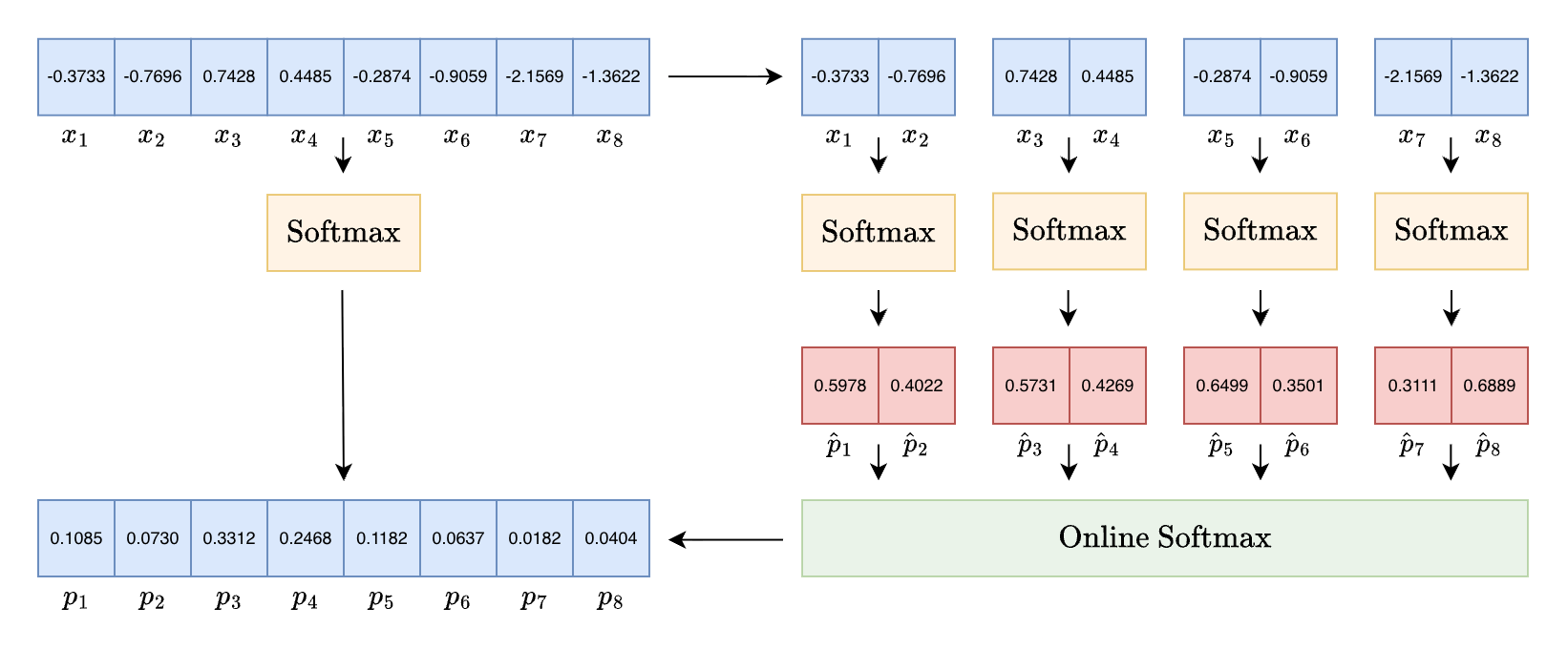
The softmax function is an crucial part of modern deep learning. It is especially important for the attention mechanism used in Transformer models. In self-attention, softmax converts raw similarity scores into a probability distribution. This distribution tells the model how much focus to put on each token in a sequence. We usually define scaled dot product attention like this:

\[\text{Attention(Q, K, V)} = \text{softmax}\left(\frac{QK^T}{\sqrt{d_k}} \right) V\]

When we calculate the dot product of queries and keys, we get an $N \times N$ a sequence of length $N$. This creates a major problem because the time and memory needed grow at a quadratic rate $O(N^2)$:

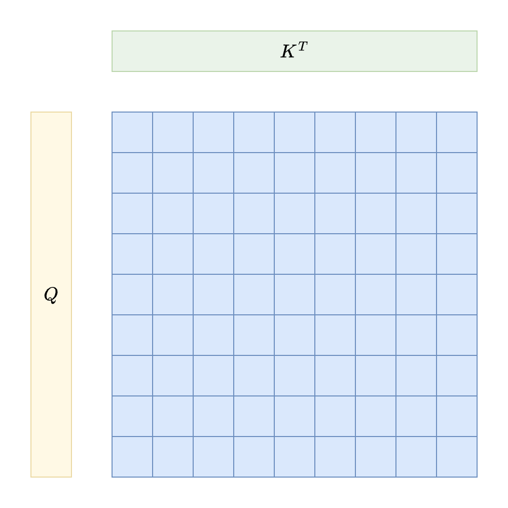
For very long sequences, a single GPU cannot store the entire attention matrix. The Ring Attention paper highlights just how extreme this memory demand can be:

To put the memory demand in perspective, even when dealing with a batch size of 1, processing 100 million tokens requires over 1000 GB of memory for a modest model with a hidden size of 1024.

To solve this, we can split the attention matrix into smaller blocks and run calculations on those blocks individually :

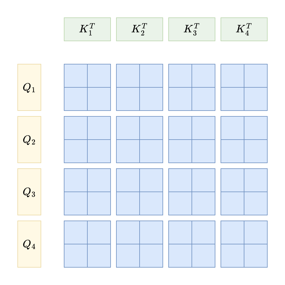
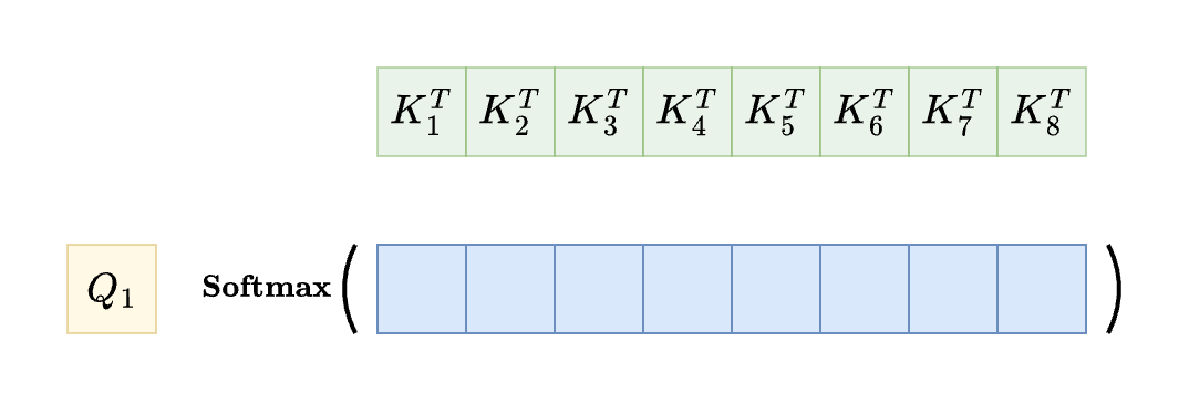
Processing in blocks is a great idea, but the standard softmax function makes it difficult because it needs the sum of every element in the sequence to calculate the denominator.

Naive Softmax

The standard softmax formula is defined as:

\[\text{Softmax}(x_i) = \frac{\exp(x_i)}{\sum_{j=1}^{N} \exp(x_j)}\]

We can write a simple version of this in PyTorch:

import torch

def naive_softmax(x: torch.Tensor) -> torch.Tensor:
    return x.exp() / x.exp().sum()

If we compare this naive function to the official PyTorch version, the results look identical for small numbers:

x         = torch.randn(8)
reference = torch.softmax(x, dim=-1)
naive     = naive_softmax(x)

print(f"Torch: {reference}")
print(f"Naive: {naive}")
print(f"allclose: {torch.allclose(reference, naive)}")

# Output
Torch: tensor([0.1085, 0.0730, 0.3312, 0.2468, 0.1182, 0.0637, 0.0182, 0.0404])
Naive: tensor([0.1085, 0.0730, 0.3312, 0.2468, 0.1182, 0.0637, 0.0182, 0.0404])
allclose: True

However, this naive version is not stable. When the input values are large, the exponential function grows too fast and causes a numerical overflow. This results in “nan” errors in naive softmax:

naive_softmax(x * 1000)

# Output
tensor([0., 0., nan, nan, 0., 0., 0., 0.])

Safe Softmax

Softmax has the shift invariance property. This means that if we add or subtract the same constant from every input, the output stays the same. We can use this to keep our numbers small and manageable. By subtracting the maximum value from the entire vector, we ensure that the largest exponent is exactly zero.

\[\begin{align*} \text{SafeSoftmax}(x_i) &= \frac{\exp(x_i)}{\sum_{j=1}^{N} \exp(x_j)} \cdot \frac{\exp(- \max_{k=1}^{N} x_k)}{\exp(- \max_{k=1}^{N} x_k)} \\\\ &= \frac{\exp(x_i - \max_{k=1}^{N} x_k)}{\sum_{j=1}^{N} \exp(x_j - \max_{k=1}^{N} x_k)} \end{align*}\]

By doing this, every exponent is less than or equal to zero, which completely prevents overflow. Here is how we implement it:

def safe_softmax(x: torch.Tensor) -> torch.Tensor:
    m = x.max()
    return (x - m).exp() / (x - m).exp().sum()

reference = torch.softmax(x, dim=-1)
safe      = safe_softmax(x)

print(f"Torch: {reference}")
print(f"Safe: {safe}")
print(f"allclose: {torch.allclose(reference, safe)}")

# Output
Torch: tensor([0.1085, 0.0730, 0.3312, 0.2468, 0.1182, 0.0637, 0.0182, 0.0404])
Safe: tensor([0.1085, 0.0730, 0.3312, 0.2468, 0.1182, 0.0637, 0.0182, 0.0404])
allclose: True

This version is also stable for large inputs:

safe_softmax(x * 1000)

# Output
tensor([0., 0., 1., 0., 0., 0., 0., 0.])

Online Softmax

In the attention mechanism, we apply softmax row by row. To calculate the denominator for a single query, we need to access every single key vector in that row. This global dependency is exactly what makes it hard to process the matrix in chunks:

Online softmax allows us to calculate the result step by step. If we track the local maximum $m$ and the local sum $d$ for each small block, we can update them as we move through the sequence. When we receive a new element $x_S$, we update our statistics like this:

\[\begin{align*} m_S &\leftarrow \max(m_{S-1}, x_S) \\ d_S &\leftarrow d_{S-1} \cdot\exp(m_{S-1} - m_S) + \exp(x_{S} - m_S) \end{align*}\]

Click for the proof

\[\begin{align*} m_S &\leftarrow \max(m_{S-1}, x_S) \\ &= \max(\max_{k=1}^{S-1} x_k, x_S) \\ &= \max_{k=1}^{S} x_k \\\\ d_S &\leftarrow d_{S-1} \cdot\exp(m_{S-1} - m_S) + \exp(x_{S} - m_S) \\ &= \left(\sum_{j=1}^{S-1} \exp(x_j - {\color{red} \cancel{m_{S-1}}}) \right) \cdot \exp({\color{red} \cancel{m_{S-1}}} - m_S) + \exp(x_{S} - m_S) \\ &= \left(\sum_{j=1}^{S-1} \exp(x_j - m_{S}) \right) + \exp(x_{S} - m_S) \\ &= \sum_{j=1}^{S} \exp(x_j - m_{S}) \end{align*}\]

This logic allows us to merge several local results into one global distribution. If we have $B$ blocks, each with its own max value $m_i$ and sum $d_i$, we can combine them by rescaling the local probabilities. This approach perfectly matches the standard softmax output:

\[\begin{align*} \text{OnlineSoftmax}(p_i, m_i, d_i) &= \frac{p_i \cdot d_i \cdot \exp(m_i -\max_{k=1}^{B})}{\sum_{j=1}^B d_j \cdot \exp(m_j - \max_{k=1}^{B})} \\ \end{align*}\]

Click for the proof

\[\begin{align*} \text{OnlineSoftmax}(p_i, m_i, d_i) &= \frac{p_i \cdot d_i \cdot \exp(m_i -\max_{k=1}^{B})}{\sum_{j=1}^B d_j \cdot \exp(m_j - \max_{k=1}^{B})} \\\\ &= \frac{\frac{\exp(x_i - m_i)}{{\color{red} \cancel{d_i}}} \cdot {\color{red} \cancel{d_i}} \cdot \exp(m_i -\max_{k=1}^{B})}{\sum_{j=1}^B d_j \cdot \exp(m_j - \max_{k=1}^{B})} \\\\ &= \frac{\exp(x_i - {\color{red} \cancel{m_i}}) \cdot \exp({\color{red} \cancel{m_i}} -\max_{k=1}^{B})}{\sum_{j=1}^B d_j \cdot \exp(m_j - \max_{k=1}^{B})} \\\\ &= \frac{\exp(x_i -\max_{k=1}^{B})}{\sum_{j=1}^B d_j \cdot \exp(m_j - \max_{k=1}^{B})} \\\\ &= \frac{\exp(x_i -\max_{k=1}^{B})}{\sum_{j=1}^B \left[\sum_{l=1}^{S_j} \exp(x_l - {\color{red} \cancel{m_i}}) \right] \cdot \exp({\color{red} \cancel{m_i}} - \max_{k=1}^{B})} \\\\ &= \frac{\exp(x_i -\max_{k=1}^{B})}{\sum_{j=1}^N \exp(x_j - \max_{k=1}^{B})} \quad\quad\quad \left(N = \sum_{j=1}^{B} S_j \right) \\ \end{align*}\]

We first need a modified version of safe softmax that returns the local maximum and the denominator sum:

def safe_softmax2(x: torch.Tensor) -> torch.Tensor:
    m = x.max()
    a = (x - m).exp() # subtract maximum value
    d = a.sum() # normalization factor
    return a / d, m, d

Next, we create the online softmax function. It takes these local blocks and merges them by finding a global maximum and adjusting the sums accordingly:

def online_softmax(
    *blocks: Tuple[torch.Tensor, torch.Tensor, torch.Tensor]
) -> torch.Tensor:
    p_blocks, m_blocks, d_blocks = zip(*blocks)
    m_max = torch.stack(m_blocks).max() # get global maximum
    d_total = sum( # compute global normalizer
        d * torch.exp(m - m_max)
        for d, m in zip(d_blocks, m_blocks)
    )
    return torch.cat(
        [
            p * d * torch.exp(m - m_max) / d_total
            for p, m, d in zip(p_blocks, m_blocks, d_blocks)
        ]
    )

Finally, we can verify that splitting the input into four chunks and processing them with our online softmax function gives the correct result:

blocks = []

for chunk in list(x.chunk(4)):
    blocks.append(safe_softmax2(chunk)) # compute p, m, d values per chunk

online = online_softmax(*blocks)

print(f"Torch: {reference}")
print(f"Online: {online}")
print(f"allclose: {torch.allclose(reference, online)}")

# Output
Torch: tensor([0.1085, 0.0730, 0.3312, 0.2468, 0.1182, 0.0637, 0.0182, 0.0404])
Online: tensor([0.1085, 0.0730, 0.3312, 0.2468, 0.1182, 0.0637, 0.0182, 0.0404])
allclose: True

Optimized Online Softmax

We can make this even more efficient . Instead of tracking the max value and the sum separately, we can combine them into a single value called the logarithm of the sum of exponentiated values or Log Sum Exp (LSE). We define this as $\text{lse}_i = m_i + \log(d_i)$. This simplifies our global formula significantly:

\[\begin{align*} \text{OnlineSoftmax}(p_i, \text{lse}_i) &= p_i \cdot \frac{\exp(\text{lse}_{i})}{\sum_{j=1}^{B} \exp(\text{lse}_j)} \end{align*}\]

Click for the proof

\[\begin{align*} \text{OnlineSoftmax}(p_i, \text{lse}\_i) &= p_i \cdot \frac{\exp(\text{lse}_{i})}{\sum_{j=1}^{B} \exp(\text{lse}_j)} \\\\ &= \frac{\exp(x_i - {\color{orange} \cancel{m_i}})}{{\color{red} \cancel{d_i}}} \cdot \frac{\exp({\color{orange} \cancel{m_i}}) \cdot {\color{red} \cancel{d_i}}}{\sum_{j=1}^{B} \exp(m_j) \cdot d_j} \\\\ &= \frac{\exp(x_i)}{\sum_{j=1}^{B} \exp(m_j) \cdot \left[\sum_{l=1}^{S_j} \exp(x_l - m_j)\right]} \\\\ &= \frac{\exp(x_i)}{\sum_{j=1}^{B} \sum_{l=1}^{S_j} \exp(x_l - {\color{red} \cancel{m_j}} + {\color{red} \cancel{m_j}} )} \\\\ &= \frac{\exp(x_i)}{\sum_{j=1}^{N} \exp(x_j)} \quad\quad\quad \left(N = \sum_{j=1}^{B} S_j \right) \end{align*}\]

To use this approach, we slightly modify the safe_softmax function so that it also returns the lse value instead of m and d separately:

def safe_softmax3(x: torch.Tensor) -> torch.Tensor:
    m = x.max()
    a = (x - m).exp()
    b = a.sum()
    lse = m + torch.log(b)
    return a / b, lse # return local softmax and lse outputs

The new online softmax function now uses these LSE weights to rescale the local probabilities before joining them together:

def online_softmax2(
    p_blocks = List[torch.Tensor],
    lse_blocks = List[torch.Tensor]
) -> torch.Tensor:
    weights = torch.exp(torch.stack(lse_blocks))         
    return torch.cat([
            p * w
            for p, w in zip(p_blocks, weights)
        ]) / weights.sum()

This version still gives us the exact same output but with a cleaner mathematical structure:

p_blocks = []
lse_blocks = []

for chunk in list(x.chunk(4)):
    p, lse = safe_softmax3(chunk) # compute p, lse values per chunk
    p_blocks.append(p)
    lse_blocks.append(lse)

online2 = online_softmax2(p_blocks, lse_blocks)
print(f"Torch: {reference}")
print(f"Online2: {online2}")
print(f"allclose: {torch.allclose(reference, online2)}")

# Output
Torch: tensor([0.1085, 0.0730, 0.3312, 0.2468, 0.1182, 0.0637, 0.0182, 0.0404])
Online2: tensor([0.1085, 0.0730, 0.3312, 0.2468, 0.1182, 0.0637, 0.0182, 0.0404])
allclose: True

Practical Implementation

Although the previous generalized version is useful for computing global softmax from multiple local softmax outputs, Ring/Striped attention uses the next key/value pairs to update the softmax output at each step. As the data moves between GPUs, the hardware calculates attention for the local block and then passes it along:

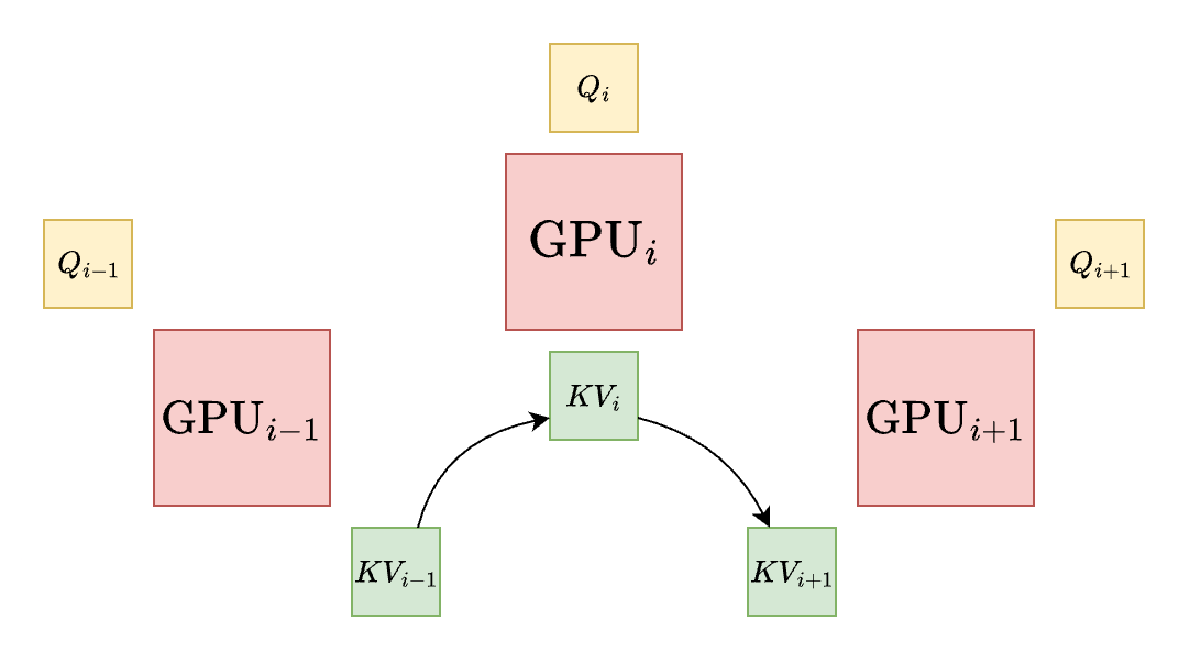
Because we are only dealing with two blocks, we can simplify the formula even further. Using the property of $\frac{1}{1 + B/A} = \frac{A}{A + B}$: we can reduce the number of times we use the exponential function:

\[\begin{align*} \text{OnlineSoftmax}(p_i, \text{lse}_i) &= p_i \cdot \frac{1}{1 + \exp(\text{lse}_{1-i} - \text{lse}_i)} \quad\quad\quad \left(i\in \\\{0,1\\\} \right) \\\\ \end{align*}\]

Click for the proof

\[\begin{align*} \text{OnlineSoftmax}(p_i, \text{lse}_i) &= p_i \cdot \frac{\exp(\text{lse}_{i})}{ \exp(\text{lse}_i) + \exp(\text{lse}_{1-i})} \quad\quad\quad \left(i\in \\\{0,1\\\} \right) \\\\ &= p_i \cdot \frac{1}{1 + \exp(\text{lse}\\_{1-i}) / \exp(\text{lse}_i)} \quad\quad \left(\frac{1}{1 + B/A} \right) \\\\ &= p_i \cdot \frac{1}{1 + \exp(\text{lse}_{1-i} - \text{lse}_i)} \end{align*}\]

Since our goal is to iteratively compute updated softmax value for given new $p$ and $lse$, we also need to compute $lse_{new}$. Since $lse_{i} = m_i + \log(d_i)$, we can find $lse_{new}$ as follows:

\[\begin{align*} \text{lse}_{\text{new}} &= \text{lse}_{0} + \log\left(1 + \exp(\text{lse}_{1} - \exp(\text{lse}_{0})) \right) \end{align*}\]

Click for the proof

\[\begin{align*} \text{lse}_{\text{new}} &= \log(\exp(\text{lse}_{0}) + \exp(\text{lse}_{1})) \\\\ &= \log\left(\exp(\text{lse}_{0}) \left[1 + \frac{ \exp(\text{lse}_{1})}{ \exp(\text{lse}_{0})} \right]\right) \\\\ &= \text{lse}_{0} + \log\left(1 + \exp(\text{lse}_{1} - \exp(\text{lse}_{0})) \right) \end{align*}\]

The implementation of this iterative update looks like this:

def online_softmax3(
    p0: torch.Tensor,
    lse0: torch.Tensor,
    p1: torch.Tensor,
    lse1: torch.Tensor
) -> tuple[torch.Tensor, torch.Tensor]:
    out0 = p0 / (1 + torch.exp(lse1 - lse0))
    out1 = p1 / (1 + torch.exp(lse0 - lse1))
    new_lse = lse0 + torch.log(1 + torch.exp(lse1 - lse0))
    return torch.cat([out0, out1]), new_lse

We can now compute the global softmax result by looping through the chunks one by one:

p, lse = p_blocks[0], lse_blocks[0]
for p_new, lse_new in zip(p_blocks[1:], lse_blocks[1:]):
    p, lse = online_softmax3(p, lse, p_new, lse_new)

print(f"Torch: {reference}")
print(f"Online3: {p}")
print(f"allclose: {torch.allclose(reference, p)}")

# Output
Torch: tensor([0.1085, 0.0730, 0.3312, 0.2468, 0.1182, 0.0637, 0.0182, 0.0404])
Online3: tensor([0.1085, 0.0730, 0.3312, 0.2468, 0.1182, 0.0637, 0.0182, 0.0404])
allclose: True

If you look at the source code for Ring Flash Attention in PyTorch, you will see a very similar pattern . They use a function to update the output and the LSE values iteratively, which allows them to handle massive sequences across multiple GPUs:

def _update_out_and_lse(
    out: torch.Tensor,
    lse: torch.Tensor,
    block_out: torch.Tensor,
    block_lse: torch.Tensor,
) -> Tuple[torch.Tensor, torch.Tensor]:
    block_out = block_out.to(torch.float32)
    block_lse = block_lse.transpose(-2, -1).unsqueeze(dim=-1)
    new_lse = lse + torch.log(1 + torch.exp(block_lse - lse))
    out = torch.exp(lse - new_lse) * out + torch.exp(block_lse - new_lse) * block_out
    lse = new_lse
    return out, lse